Chapter 2 Part 2: Tabular Models and Time-Series
2.1 Hydrograph separation
- This module was developed by Ana Bergrstrom and Matt Ross.
2.1.1 Learning Module 1
2.1.1.1 Summary
Streamflow can come from a range of water sources. When it is not raining, streams are fed by the slow drainage of groundwater. When a rainstorm occurs, streamflow increases and water enters the stream more quickly. The rate at which water reaches the stream and the partitioning between groundwater and faster flow pathways is variable across watersheds. It is important to understand how water is partitioned between fast and slow pathways (baseflow and stormflow) and what controls this partitioning in order to better predict susceptibility to flooding and if and how groundwater can sustain streamflow in long periods of drought.
In this module we will introduce the components of streamflow during a rain event, and how event water moves through a hillslope to reach a stream. We will discuss methods for partitioning a hydrograph between baseflow (groundwater) and storm flow (event water). Finally, we will explore how characteristics of a watershed might lead to more or less water being partitioned into baseflow vs. stormflow. We will test understanding through evaluating data collected from watersheds in West Virginia to determine how mountaintop mining, which fundamentally changed the watershed structure, affects baseflow.
2.1.1.2 Reading for this lab
Ladson, A. R., R. Brown, B. Neal and R. Nathan (2013) A standard approach to baseflow separation using the Lyne and Hollick filter. Australian Journal of Water Resources 17(1): 173-18
Lynne, V., Hollick, M. (1979) Stochastic time-variable rainfall-runoff modelling. In: pp. 89-93 Institute of Engineers Australia National Conference. Perth.
2.1.1.3 Overall Learning Objectives
At the end of this module, students should be able to describe the components of streamflow, the basics of how water moves through a hillslope, and the watershed characteristics that affect partitioning between baseflow and stormflow.
2.1.1.5 Components of streamflow during a rain event
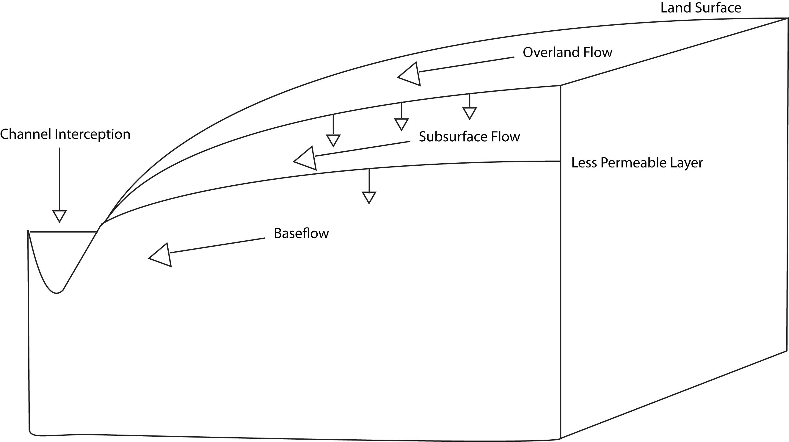
During a rainstorm, precipitation is falling across the watershed: close to the stream, on a hillslope, and up at the watershed divide. This water that falls across the watershed flows downslope toward the stream via a number of flow pathways. Here we define and describe the basic flow pathways during a rain event.
The first component is channel interception. This is water that falls directly on the water surface of the stream. The amount of water that falls directly on the channel is a function of stream size, if we have a very small, narrow creek, this will be a very small quantity. However, you can imagine that in a very large, broad river such as the Amazon, this volume of water is much larger. Channel interception is the first component during a rain event that causes streamflow to increase because it is contributing directly to the stream and therefore has no travel time.
The second is overland flow, which is water that flows on the land surface to the stream. Overland flow can occur via a number of mechanisms which we will not explore too deeply here, but encourage further study on your own (resources provided). Briefly, overland flow includes water that falls on an impermeable surface such as pavement, water that runs downslope due to rain falling faster than the rate at which it can infiltrate the ground surface, and water that flows over the land surface because the ground is completely saturated. Overland flow is typically faster than water that travels through soils and deeper flow pathways and therefore is the next major component that starts to contribute to the increase in streamflow during a rain event.
The third component is subsurface flow. This is water that infiltrates the land surface and flows downslope through shallow groundwater flow pathways. This is the last component that increases streamflow during a storm event, is the slowest of the stormflow components, and can contribute to elevated streamflow for a while after precipitation ends.
The final component is baseflow. Baseflow can also be described as groundwater. This component is what sustains streamflow between rain events, but also continues to contribute during a rain event. Of water that infiltrates the ground surface, some moves quickly to the stream as subsurface flow, but some moves deeper and becomes part of deeper groundwater and baseflow. Thus baseflow can increase in times of higher wetness in the watershed, particularly during and right after rainy seasons or spring snowmelt.
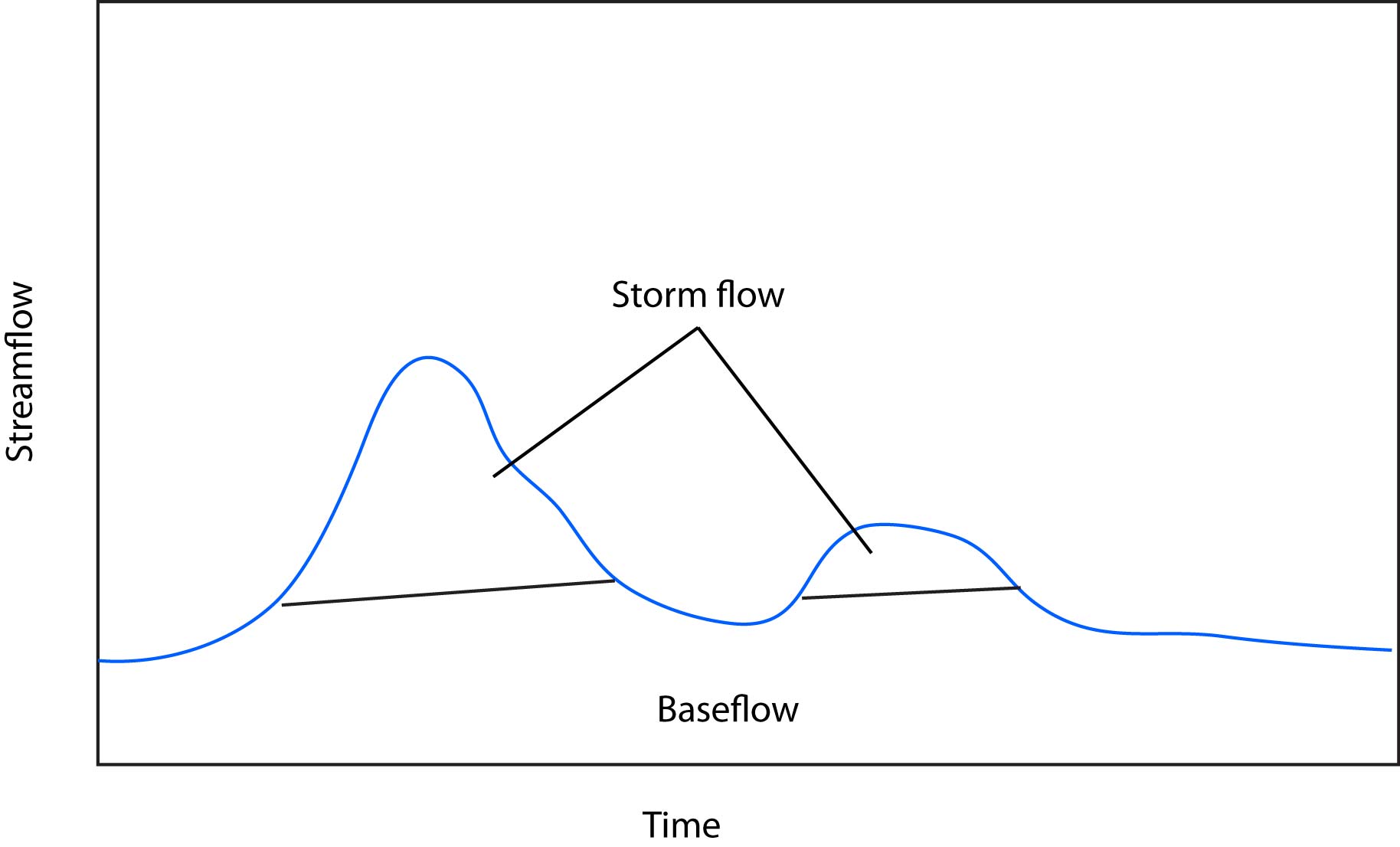
We can simplify this partitioning into baseflow and stormflow (often called quickflow). Baseflow being groundwater that moves more slowly and sustains streamflow between rain events. Stormflow is water that contributes to streamflow as a result of a rain event. Under this definition we can lump channel interception, overland flow, and subsurface flow into stormflow.
2.1.1.6 Storm flow through a hillslope
When rain falls on the land surface, much of it infiltrates into the soil. Water moves through the soil column until it meets a layer of lower permeability and runs down the hillslope as subsurface flow. This layer of lower permeability allows some water to move through it, contributing to groundwater. Frequently the layer of lower permeability is the interface between soil and rock. Therefore the depth of soil has a large effect on how much water moves through soil vs. how much moves deeper into groundwater, becoming baseflow.
2.1.1.7 How we quantify baseflow
It is impossible to know the amount of water moving as overland, subsurface, and base flow in all parts of a watershed. So in order to quantify how much water in a stream at any given time is storm flow vs. baseflow, we need to use some simplified methods (i.e., modeling). These frequently involve using the hydrograph (plot of streamflow over time) drawing lines, and calculating the volume of water above and below the line. This can be somewhat arbitrary and there are a variety of methods for delineating the cutoff between baseflow and stormflow. Despite what method you use and how simplified it is, this technique still provides valuable information and allows us to make comparisons across watersheds in order to understand how they function and what their structural properties are.
2.1.1.8 Baseflow separation methods
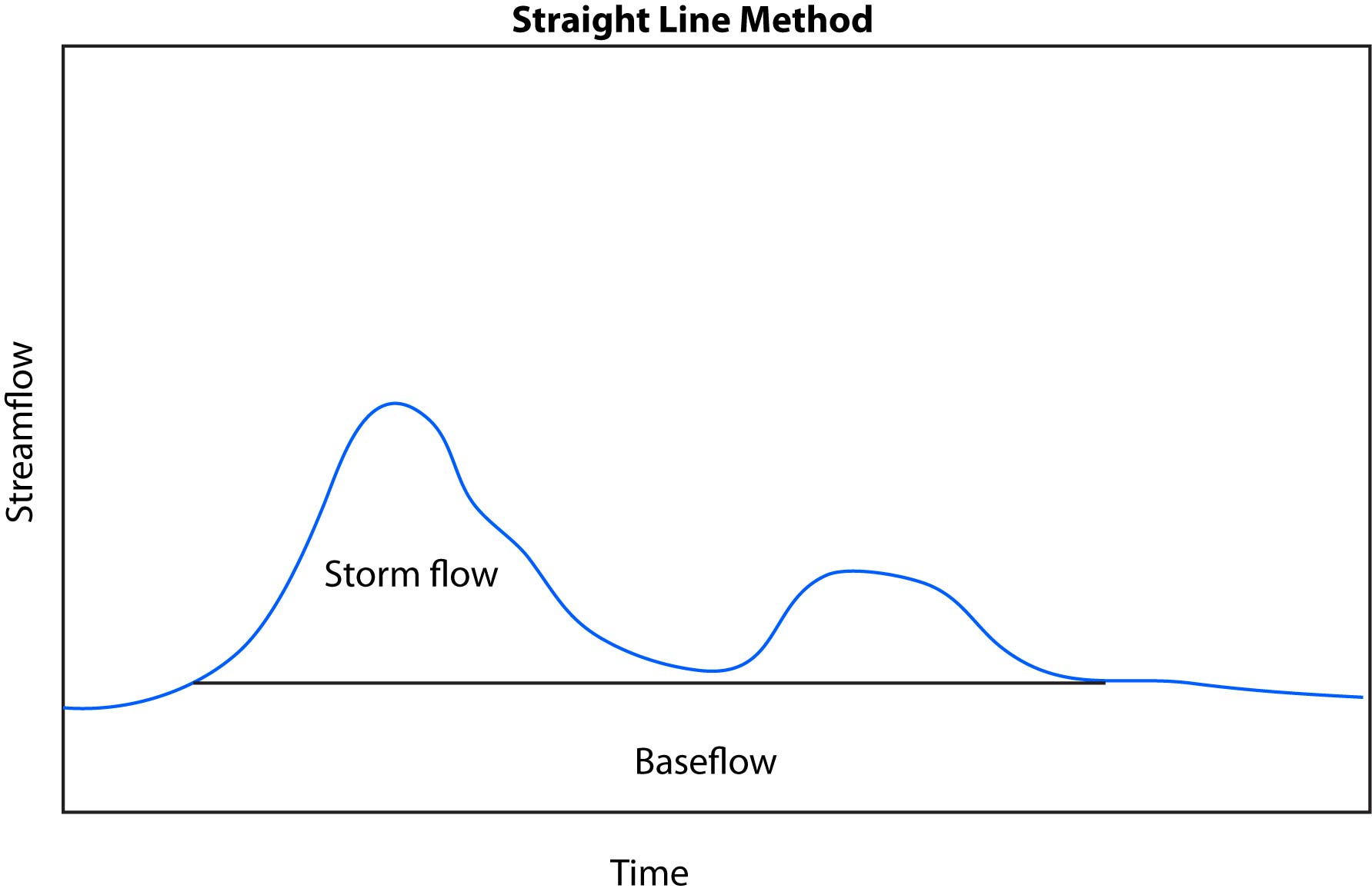
One of the most basic methods for calculating base flow vs. storm flow is the straight line method. First, find the value of discharge at the point that streamflow begins to rise due to a storm. A straight line is drawn at that value until it intersects with the hydrograph (i.e. streamflow recedes back to the discharge it was at before the rainfall event started. Anything below this line is base flow and anything above it is storm flow.
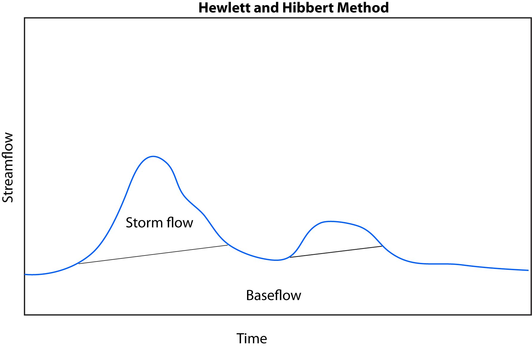
We learned above that some rainfall can move deep into the soil profile and contribute to baseflow. We might expect baseflow to increase over time and thus would want to use a method that can account for this.
An addition to the straight line method was posed by Hewlett and Hibbert, 1967. This method, which we’ll call the Hewlett and Hibbert method finds the discharge at the starting point of a storm. Then, rather than a straight line of 0 slope and in the straight line method, we assume a slope of 0.05 cubic feet per second per square mile. The line with this calculated slope is drawn until it intersects with the hydrograph receding at the end of the storm.
There are myriad other methods for baseflow separation of a wide range of complexity. We will give an example of one more method: a recursive filter method established by Lyne and Hollick (1976). This method smooths the hydrograph and partitions part of that smoothed signal into baseflow. The equation for this method is:
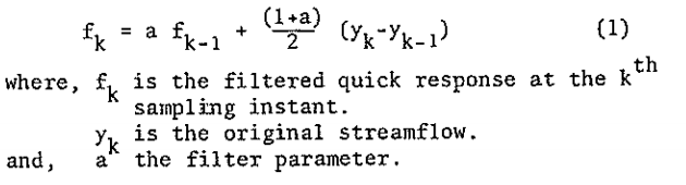
You can see from this equation that a filter parameter, a, must be chosen. This parameter can be decided by the user, takes a value between 0 and 1, and is typically close to 1. Additionally this filtering method must be constrained so that baseflow is not negative or greater than the total streamflow. Output from this method for the Harvey River in Australia is originally published in Lyne and Hollick (1976) below (notice in the caption that the a parameter was set to 0.8):
2.1.1.9 Watershed controls on baseflow and stormflow
The way a watershed is structured has a strong control on how water is partitioned into baseflow and stormflow. Below is a list of key structural properties:
Land Use and Land Cover: If a watershed is developed or natural can dictate how much water infiltrates the land surface and how quickly. For example, a watershed with lots of pavement means that much more water will be overland flow with fewer opportunities to recharge baseflow. Furthermore, how a watershed is developed will affect partitioning. For example a residential area with houses on large, grassy lots will allow for more infiltration than a shopping center with large parking lots. Land cover in natural areas will also affect partitioning. Some other variables to consider may be:
Land cover in natural areas: a dense forest vs. a recently harvested hillside.
Soil type: clayey soils vs. sandy soils
Depth to impeding layer: could be the bedrock interface, but could also be a low permeability clay layer in the soil
Permeability of the underlying rock: Highly fractured sandstone vs. solid granite
Slope: steeper slopes vs. flatter areas
The partitioning is a combination of all of these factors. A watershed may have a very low slope, suggesting that it might have less stormflow. But if the soils in this watershed have an impermeable clay layer near the soil surface, a lot more water may end up as stormflow than one would expect.
2.1.2 Labwork (20 pts)
In this lab we will analyze stream flow (Q) and precipitation (P) data from Tenderfoot Creek Experimental Forest (TCEF). TCEF is located in central Montana, north of White Sulphur Springs. See here for information about TCEF. You will do some data analysis on flows, calculate annual runoff ratios, and perform a hydrograph separation.
2.1.3 Repo link
Follow this link to download everything you need for this unit. When you get to GitHub click on “Code” (green button) and select “download zip”. You will then save this to a local folder where you should do all of your work for this class. You will work through the “_blank.Rmd” or “_partial.Rmd”. Always be sure to read the README.md files in the GitHub repo. Sometimes they are useful, sometimes they aren’t, but always have a look. As I mentioned above you will work through the “_blank.Rmd” or “_partial.Rmd”. If you want to learn how to code in R, I encourage you to work through the blank version as much as possible. Also, if you don’t have much R background this lab might seem kind of challenging. But don’t worry. I’m challenging you right now, but it will get easier, and we can video chat if a live demonstration is needed. So don’t get frustrated if this seems tough right now. Soon you will be rattling off code with ease. Conversely, if you are an experienced coder and have ideas for how to do this in ways other than what I’ve shown here, please share code with your colleagues and help them develop their coding skills!
Once you have this folder saved where you would like it, open RStudio and navigate to the folder. Next, open the project (“.Rproj”). Doing so will set the folder as the working directory, make your life easier, and make everything generally work. The use of projects is highly recommended and is the practice we will follow in this class. See here for an overview of projects and why you should use them from Jenny Bryan.
2.2 Return Intervals
- In this learning module we will focus on return intervals. We first need to understand return intervals before we can move onto the rational method and curve numbers.
The repo for this module can be found here
2.2.1 Learning Module 2
2.2.1.1 Background information
Lecture from colleague Joel Sholtes on precipitation frequency analysis.
Short lecture on Intensity-Duration-Frequency (IDF) curves
Reading on frequency analysis of flow (e.g., floods). You should notice that the frequency analysis is the same whether we apply it to Q (flow) or P (precipitation). So as long as you understand the fundamental principles you will be able to do frequency analysis on either Q or P.
USGS reading on flow frequency analysis
There are also probability lecture slides on D2L. Titled “probability.pptx”.
2.2.2 Labwork (20 pts)
In this lab we will look at some precipitation data to get an idea of return intervals for a given rain event. A return interval is the inverse of the probability. So if a certain rain even has a 10% probability of happening any year it has a 1/p return interval, so: R = 1/0.1 = 10 years. This means on average you can expect that size event about every ten years. From a probability perspective it is actually more correct to state that there is a 10% chance of that size rain event in any year. The reason this is better is that it communicates that you certainly can have a 10% probability event occur in back-to-back years.
After computing some return intervals we will then use some of the simpler rainfall-runoff modeling approaches (the rational method and the curve number method) to simulate runoff for a hypothetical basin in our next unit.
This is knitr settings. Knitr is a package that will turn this Rmd to an html.
2.2.2.1 Packages
We have a few new packages today. Those include rnoaa and leaflet. rnooa is a package used to download NOAA climate data. leaflet is a package for interactive mapping.
Recall that if you have not installed these packages on your computer you will need to run:
install.packages(“rnoaa”) and so on for the others.
2.2.2.2 Precipitation return intervals
First, let’s start by getting some precipitation (P) data. rnoaa has a function called ghcnd_stations(). This function will download the site information for all stations in the GHCND network.
GHCND network - Link
Ok, so we want station USC00241044, which runs from 1892 to now. We use the meteo_pull_monitors() function to do that.
Now we have some climate data. Take a minute to look at the climate_data df. First, just looking at the df we see that the data don’t actually start until 1894. It is also always a good idea to just plot some data. Below plot prcp, snow, tmax and tmin. You can just make 4 different plots. This is just for visual inspection. This part of the process is called exploratory data analysis (EDA). This should always be the first step when downloading data whether you download the data from the internet or from a sensor in the field.
You might have noticed that the values seem to be much too large! Did you notice that? This is a great skill to develop. Have a look at the data and ask “are these numbers reasonable?”. In this case, the answer would be no!
One thing to note is that NOAA data comes in tenths of degrees for temp and tenths of millimeters for precip. Type ?meteo_pull_monitors into the console and the help screen will tell you that. So, we need to clean up the df a bit. Let’s do that here.
Now that we’ve converted units, it is a good idea to plot your data again for some EDA. Make plots of each of the variables (prcp, snow, tmax, and tmin) over time to inspect.
How do the data look? Do they make sense? Do you see any strange values?
There is a large snow event in 1951. We can assume that is “real”, so let’s keep it in the analysis. But you should think through how you could exclude it from the analysis. How could you use the filter function to do that?
Next, we want to use some skills from the hydrograph sep lab to add a water year (WY) column. Try that here.
I like to rearrange the order of columns. Using:
Now, create a new df called climate_an where you calculate the total P (i.e., the sum) for each water year. Use group_by and summarize (or better yet, reframe). Also keep in mind that you will need to deal with NA values in the df. How do you do that in summarize? As a note, reframe can be used instead of summarize and is a more general purpose function. You can try each.
What happens if you don’t deal with NA values by using something like na.rm = TRUE?
Now, plot total anual P on the Y and water year on the x. What do you see?
Now let’s calculate some probabilities. Look up the pnorm() function for this (either type it into the Help window, or type ?pnorm in the console. You only need x, the mean, and standard deviation (sd) for the calculations.
Q1. (3 pts) What is the probability that the annual precipitation in a given year is less than 400 mm? This is the F(A) in the CDF in the probability lecture slides.
Q1 ANSWER:
Q2. (3 pts) What is the probability that the maximum annual precipitation in a given year is GREATER than 500 mm?
Q2 ANSWER:
Q3. (3 pts) What is the probability that the annual P is between 400 and 500 mm?
Q4. (3 pts) What is the return period for a year with AT LEAST 550 mm of precip? The return period, Tr, is calculated as Tr = 1/p, with p being the probability for an event to occur.
Q5. (8 pts) Explain why probability analysis of climate data assumes the data are normally distributed and stationary? Below provide a histogram and a density plot of the total annual P data and comment on the visual appearance in terms of normality. Next use google and the links below to test for normality and stationarity. Be quantitative in commenting on the normality and stationarity of the total P data.
2.3 Rational method and NRCS curve number (20 pts)
The repo for this module can be found here
2.3.1 Learning Module 3
2.3.1.1 Background information - Rational Method
The Rational Method is a type of simple hydrological analysis used to estimate the peak runoff rate from a small watershed during a rainfall event. It is particularly useful for estimating the amount of water that will flow through a particular area during a storm, like a drainage system or culvert. Despite the existence of more advanced methods, this approach remains widely used in practice for its simplicity and ability to provide quick approximations, making it invaluable for preliminary assessments and as a foundation for understanding more complex hydrological and environmental modeling techniques.
Here is a 5-minute video to get started:
2.3.1.2 Reading - Rational Method.
Read at least sections 2 and 3 to for the formula and an example
Some helpful terminology:
runoff coefficient - represents how much rainfall actually becomes runoff
time of concentration - the time it takes for some mass of precipitation to travel from the most remote point in a watershed to the outlet or point of interest. e.g., how long it takes a drop of rain to reach a culvert after it falls to the ground.
2.3.1.3 Background information - Curve Number
The NRCS (Natural Resources Conservation Science) curve number (CN) is a tool used to estimate the total runoff volume of water that will run off an ungaged watershed during a storm event. The curve number is based on soil type, land use and antecedent moisture conditions. You may also see SCS CN in texts. NRCS was previously known as Soil Conservation Science, they are the same. It was designed as a simple tool to describe typical watershed response from infrequent rainfall anywhere in the US for watersheds with the same soil type, land use, and surface runoff conditions. The CN method is a single event model to estimate of runoff volume from rainfall events (not peak discharge or a hydrograph).
To understand the function and derivation of the CN number, let’s start with the
the NRCS runoff equation:
\[
Q = \frac{{(P - I_{a})^2}}{{P - I_{a} + S}}
\]
Where Q = runoff(in)
P = rainfall (in)
S = potential maximum retention after runoff begins
Ia = initial abstraction (initial amount of rainfall that is intercepted by the watershed surface and does not immediately contribute to runoff)
Ia is assumed to reduce to 0.2S based on empirical observations by NRCS. If: \[ S = \frac{{1000}}{{CN}} - 10 \] the runoff equation therefore reduces to: \[ Q = \frac{{[P - 0.02\left(\frac{{1000}}{{CN}} - 10\right)]^2}}{{P + 0.8\left(\frac{{1000}}{{CN}} - 10\right)}} \]
2.3.1.4 Reading - Curve numbers
Curve Number selection tables are available from the US Army Corps.
Slides on selecting curve number start around slide 8.
- Link
2.3.1.5 Reading - Supporting material
Time of concentration. Up to “other considerations”, pages 15-1 to 15-9.
- Link
We will use the Kirpich method to calculate the time of concentration. Here is the citation for your reference.
Kirpich, Z.P. (1940). “Time of concentration of small agricultural watersheds”. Civil Engineering. 10 (6): 362.
2.3.2 Labwork (20 pts)
In this module, you will apply the Rational Method and the SCS curve number (CN) method to estimate peak flows and effective rainfall/runoff volumes. This lab also introduces two coding techniques; for-loops and functions.
This is knitr settings. Knitr is a package that will turn this Rmd to an html.
Packages
2.3.2.1 Part I - Rational Method
The goal is to calculate peak runoff (cfs) for a small 280-acre rangeland watershed near Bozeman for multiple events with different return periods. You will first have to calculate the time of concentration and then look up the the rainfall values for the different return intervals. The longest flowpath in the watershed is 6300 ft long, average watershed slope is 1.95%. Look at this table to select C.
2.3.2.1.1 Time of Concentration
- Time of concentration is the time it takes water to travel along the longest flowpath in the watershed and exit the watershed.
tc in this example should be ~ 29.91. If your calculated value is very different, start by checking slope value (S). For the sake of simplicity in next steps, do not change the name of variables.
2.3.2.1.2 Storm Depths
Now that you have the time of concentration, you need to find the corresponding 1, 2, 5, 10, 25, 50, and 100 year storm depths for a duration that works for the Rational Method in that particular watershed (that is, the duration that is closest to tc). Create a dataframe (or ‘tibble’ which is the tidyverse data frame) called “storms” that has a column for the return period, Tr, the storm depth, Pin, and the average storm intensity over ONE HOUR, Pin_hr. Typically hourly depths may be determined from a rainfall analysis. For the sake of the assignment, approximate daily depths corresponding to appropriate frequencies are provided here for Bozeman, MT. To obtain 1 hour depths by dividing daily depth by 24.
2.3.2.1.3 Example for-loop
Now that we have the rainfall intensities, we need to set up a way that calculates Qp for each of those intensities, without us having to go back and manually enter them each time. We do this with a for-loop. Let’s first look at how for loops work in R.
A for-loop will execute the code inside it for a specified number of iterations. The structure looks like: for(i in some number of iterations) { output <- some code/function that needs to be executed } In the chunk below, we create the vector x, which contains 6 values (0, 2, 4, 6, 8, 10). Each loop then executes a calculation using each value in ‘x’ in sequence. In a for-loop, ‘i’ is called the loop index or iterator. It has a new value in each iteration of the loop. You can think of i as a ‘counter’ that helps the loop keep track of its progress. In the example below, we want to run the code in the loop for every value in the vector ‘x’. Since there are 6 values in vector ‘x’, then we will tell the loop to run 6 times. However, rather than for (i in 1:6), using 1:length(x) ensures the loop adapts to the size of x, no matter how many values it contains. This improves the flexibility of our code. We also need to store the output of loop during each iteration. If we don’t store the results of each iteration or loop, the loop will overwrite the output each time, leaving us with only the result from the final iteration. To store the output of each loop iteration, we have to preallocate a vector (like y) to store all of the outputs. In other words, we are creating an empty vector with the same length as ‘x’ for the for-loop to add values to.
We have created a vector x from 0 to 10 in increments of 2. The for-loop takes each element of that vector and squares it. The “i” is called an index and runs from 1 through 6 (the length of x). During the first iteration i is 1, during the second iteration i is 2, and so on. We are then writing the results from the calculation into a new vector, y. When i is 1, we are squaring the first value in vector x, which is 0. The first value in y will be zero as well. When i is 2, the second value in x gets squared, which is 2^2. The second value in y is going to be 4.
2.3.2.1.4 Calculate Qp with for-loop
Now let’s set up the for-loop for the Rational Method. We need to set up a for-loop that does the same calculation 7 times, the number of precip values in “storms”. However, ‘length()’ for a dataframe returns the number of columns, so you want to use ‘nrow()’ when referencing a dataframe. (As apposed to using length() for a vector as above). The calculated peak discharges should go into a new column of our “storms” df. However, indexing is slow for dataframes, so we will write the new values into a new vector, Qp, and then after the loop insert the vector as a column into the dataframe.
If you are using the complete version of the assignment, do not assume that this C value is correct
2.3.2.1.5 Plot Tr and Qp
Now plot the return interval against the storm peakflow. You only need three to four lines for this: 1st sets up the data, 2nd defines the theme that removes the gray background and sets the axes labels to a proper size, 3rd plots the data with geom_points, 4th makes the axes labels with labs. Note that axis labels have units. This is an important feature when communicating your findings.
1. (1 pt) What does the C in the Rational Method do?
ANSWER:
2. (2 pt) What is the the time of concentration and why does it need to be taken into account for the Rational Method? What is a common issue among many tc methods?
ANSWER:
2.3.2.2 Part II - NRCS CN
In this exercise we will write a function that takes the necessary inputs for the NRCS CN method and returns a value based on the parameters. This is not fully automated, you will still have to look up the CN yourself for a given land use. The goal is to write a function that requires P, CN, and AMC (antecedent moisture condition) as an input in order to calculate Q.
2.3.2.3 Function example
Let’s look at a simple example for a function. Assume we want a number with an exponent and we want to be able to choose both the base and the exponent. The function ‘function()’ defines the inputs in (), the actual calculation then follows in {}.
Run the above function. You will notice that a function was added to the Global Environment all the way at the bottom. Now let’s test the function with a base of 2 and an exponent of 3. This should perform the calculation 2x2x2 = 8
2.3.2.3.1 NRCS CN test
Before we write a function to estimate Q using CN, let’s make sure we can set up the correct steps WITHOUT the function. This is almost always a helpful step in developing functions. It can save hours of headaches later. Let’s try P = 2.5 inches, CN = 90, and AMC = 3. The biggest problem here is going to be creating a lookup table for the AMC. I will provide the basic structure of the code for this.
Sanity check: Q should ~ 2.0 for the specified parameters.
3. (4 pt) What is one of the critical assumptions for the SCS CN method? (1-2 sentences). Why is it important to understand assumptions of models like this one?
ANSWER:
Now write a function called “scs_cn” that takes the inputs P, CN, and AMC (all numeric) and returns Q, Ia, Si, and the RR as a df called “scs_out”. Test the function for P = 2.5 in, CN = 90, AMC = 3.
4. (4 pts) Describe what factors into the curve number (and most notably what is missing). What does it mean when the CN is 100 or 0?
ANSWER:
5. (3 pts) What is the difference between a deterministic and a stochastic model? Describe one example each.
ANSWER:
6. (6 pts)(4-6 sentences) Let’s consider the cross-disciplinary relevance of hydrological modeling. You may not be studying hydrology directly, but environmental resource managers often need to estimate peak flows. Why? (1-2 sentences). In a sentence, what is your specific area of interest, or the topic of your professional paper, if known. Consider broader implications of the hydrologic cycle, like water quality, nutrient or pollution transport, or erosion. Does rainfall/runoff management affect your niche? If so, how? (2-4 sentences) ANSWER:
2.4 Transfer function rainfall-runoff models
2.4.1 Learning Module
2.4.1.1 Summary
In previous modules, we explored how watershed characteristics influence the flow of input water through or over hillslopes to quickly contribute to stormflow or to be stored for later contribution to baseflow. Therefore, the partitioning of flow into baseflow or stormflow can be determined by the time it spends in the watershed. Furthermore, the residence time of water in various pathways may affect weathering and solute transport within watersheds. To improve our understanding of water movement within a watershed, it can be crucial to incorporate water transit time into hydrological models. This consideration allows for a more realistic representation of how water moves through various storage compartments, such as soil, groundwater, and surface water, accounting for the time it takes for water to traverse these pathways.
In this module, we will model the temporal aspects of runoff response to input using a transfer function. First, please read:
TRANSEP - a combined tracer and runoff transfer function hydrograph separation model
Then this chapter will step through key concepts in the paper to facilitate hands-on exploration of the rainfall-runoff portion of the TRANSEP model in the assessment. Then, we will introduce examples of other transfer functions to demonstrate alternative ways of representing time-induced patterns in hydrological modeling, prompting you to consider response patterns in your study systems.
2.4.1.2 Overall Learning Objectives
At the end of this module, students should be able to describe several ways to model and identify transit time within hydrological models. They should have a general understanding of how water transit time may influence the timing and composition of runoff.
2.4.1.3 Terminology
In modeling a flow system, note that consideration of time may vary depending on the questions being asked. Transit time is the average time required for water to travel through the entire flow system, from input (e.g., rainfall on soil surface) to output (e.g., discharge). Residence time is a portion of transit time, describing the amount of time water spends within a specific component of the flow system, like storage (e.g., in soil, groundwater, or a lake).

A transfer function (TF) is a mathematical representation of how a system responds to input signals. In a hydrological context, it describes the transformation of inputs (e.g. precipitation) to outputs (e.g. runoff). These models can be valuable tools for understanding the time-varying dynamics of a hydrological system.
2.4.1.4 The Linear Time-Invariant TF
We’ll begin the discussion in the context of a linear reservoir. Linear reservoirs are simple models designed to simulate the storage and discharge of water in a catchment. These models assume that the catchment can be represented as single storage compartments or as a series of interconnected storage compartments and that the change the amount of water stored in the reservoir (or reservoirs) is directly proportional to the inflows and outflows. In other words, the linear relationship between inflows and outflows means that the rate of water release is proportional to the amount of water stored in the reservoir.
2.4.1.4.1 The Instantaneous Unit Hydrograph:
The Instantaneous Unit Hydrograph (IUH) represents the linear rainfall-runoff model used in the TRANSEP model. It is an approach to hydrograph separation that is useful for analyzing the temporal distribution of runoff in response to a ‘unit’ pulse of rainfall (e.g. uniform one-inch depth over a unit area represented by a unit hydrograph). In other words, it is a hydrograph that results from one unit (e.g. 1 mm) of effective rainfall uniformly distributed over the watershed and occurring in a short duration. Therefore, the following assumptions are made when the IUH is used as a transfer function:
1. the IUH reflects the ensemble of watershed characteristics
2. the shape characteristics of the unit hydrograph are independent of time
3. the output response is linearly proportional to the input

By interpreting the IUH as a transfer function, we can model how the watershed translates rainfall into runoff. In the TRANSEP model, this transfer function is represented as \(g(\tau)\) and thus the rainfall-induced response to runoff.
\[
g(\tau) = \frac{\tau^{\alpha-1}}{\mathrm{B}^{\alpha}\Gamma(\alpha)}exp(-\frac{\tau}{\alpha})
\]
The linear portion of the TRANSEP model describes a convolution of the effective precipitation and a runoff transfer function.
\[
Q(t)= \int_{0}^{t} g(\tau)p_{\text{eff}}(t-\tau)d\tau
\]
Whoa, wait…what? Tau, integrals, and convolution? Don’t worry about the details of the equations. Check out this video to have convolution described using dollars and cookies, then imagine each dollar as a rainfall unit and each cookie as a runoff unit. Review the equations again after the video.
2.4.1.4.2 The Loss Function:
The loss function represents the linear rainfall-runoff model used in the TRANSEP model.
\[
s(t) = b_{1} p(t + 1 - b_{2}^{-1}) s(t - \triangle t)
\]
\[
s(t = 0) = b_{3}
\]
\[
p_{\text{eff}}(t) = p(t) s(t)
\]
where \(p_{\text{eff}}(t)\) is the effective precipitation.
\(s(t)\) is the antecedent precipitation index which is determined by giving more importance to recent precipitation and gradually reducing that importance as we go back in time.
The rate at which this importance decreases is controlled by the parameter \(b_{2}\).
The parameter \(b_{3}\) sets the initial antecedent precipitation index at the beginning of the simulated time series.
In other words, these equations are used to simulate the flow of water in a hydrological system over time. The first equation represents the change in stored water at each time step, taking into account precipitation, loss to runoff, and the system’s past state. The second equation sets the initial condition for the storage at the beginning of the simulation. The third equation calculates the effective precipitation, considering both precipitation and the current storage state.
2.4.1.4.3 How do we code this?
We will use a skeletal version of TRANSEP, focusing only on the rainfall-runoff piece which includes the loss-function and the gamma transfer function.
We will use rainfall and runoff data from TCEF to model annual streamflow at a daily time step. Then we can use this model as a jump-off point to start talking about model calibration and validation in future modules.
2.4.1.4.4 Final thoughts:
If during your modeling experience, you find yourself wading through a bog of complex physics and multiple layers of transfer functions to account for every drop of input into a system, it is time to revisit your objectives. Remember that a model is always ‘wrong’. Like a map, it provides a simplified representation of reality. It may not be entirely accurate, but it serves a valuable purpose. Models help us understand complex systems, make predictions, and gain insights even if they are not an exact replica of the real world. Check out this paper for more:
https://agupubs.onlinelibrary.wiley.com/doi/10.1029/93WR00877
2.4.3 Download the repo for this lab HERE
In this homework/lab, you will write a simple, lumped rainfall-runoff model. The foundation for this model is the TRANSEP model from Weiler et al., 2003. Since TRANSEP (tracer transfer function hydrograph separation model) contains a tracer module that we don’t need, we will only use the loss function (Jakeman and Hornberger) and the gamma transfer function for the water routing.
The data for the model is from the Tenderfoot Creek Experimental Forest in central Montana.
Load packages with a function that checks and installs packages if needed:
Define input year We could use every year in the time series, but for starters, we’ll use 2006. Use filter() to extract the 2006 water year.
1) QUESTION: What does the function cumsum() do?(1 pt) ANSWER:
Define the initial inputs
This chunk defines the initial inputs for measured precip and measured runoff.
Parameterization
We will use these parameters. You can change them if you want, but I’d suggest leaving them like this at least until you get the model to work. Even tiny changes can have a huge effect on the simulated runoff.
Loss function
This is the module for the Jakeman and Hornberger loss function where we turn our measured input precip into effective precipitation (p_eff). This part contains three steps.
1) preallocate a vector p_eff: Initiate an empty vector for effective precipitation that we will fill in with a loop using Peff(t) = p(t)s(t). Effective precipitation is the portion of precipitation that generates streamflow and event water contribution to the stream. It is separated to produce event water and displace pre-event water into the stream.
2) set the initial value for s: s(t) is an antecedent precipitation index. How much does antecedent precipitation affect effective precipitation?
3) generate p_eff inside of a for-loop
Please note: The Weiler et al. (2003) paper states that one of the loss function parameters (vol_c) can be determined from the measured input. That is actually not the case.
s(t) is the antecedent precipitation index that is calculated by exponentially weighting the precipitation backward in time according to the parameter b2 is a ‘dial’ that places weight on past precipitation events.
2) QUESTION (3 pts): Interpret the two figures. What is the meaning of “frac”? For this answer, think about what the effective precipitation represents. When is frac “high”, when is “frac” low?
ANSWER:
Extra Credit (2 pt): Combine the two plots into one, with a meaningfully scaled secondary y-axis
Runoff transfer function
Routing module -
This short chunk sets up the TF used for the water routing. This part contains only two steps: 1) the calculation of the actual TF. 2) normalization of the TF so that the sum of the TF equals 1.
tau(0) is the mean residence time
3) QUESTION (2 pt): Why is it important to normalize the transfer function?
ANSWER:
4) QUESTION (4 pt): Describe the transfer function. What are the units and what does the shape of the transfer function mean for runoff generation?
ANSWER:
Convolution
This is the heart of the model. Here, we convolute the input with the TF to generate runoff. There is another thing you need to pay attention to: We are only interested in one year (365 days), but since our TF itself is 365 timesteps long, small parts of all inputs except for the first one, will be turned into streamflow AFTER the water year of interest, that is, in the following year. In practice, this means you have two options to handle this.
1) You calculate q_all and then manually cut the matrix/vector to the correct length at the end, or
2) You only populate a vector at each time step and put the generated runoff per iteration in the correct locations within the vector. For this to work, you would need to trim the length of the generated runoff by one during each iteration. This approach is more difficult to code, but saves a lot of memory since you are only calculating/storing one vector of length 365 (or 366 during a leapyear).
We will go with option 1). The code for option 2 is shown at the end for reference.
Convolution summarized (recall dollars and cookies): Each loop iteration results in a row of the matrix representing the convolution at a specific time step. each time step of p_eff is an iteration, and for each timestep, it multiplies the effective precipitation at that timestep by the entire transfer function. Then each row is summed and stored in the vector q_all. q_all_loop is an intermediate step in the convolution process and can help visualize how the convolution evolves over time. As an example, if we have precip at time step 1, we are interested in how this contributes to runoff at time steps 1,2,3 etc, all the way to 365 (or the end of our period). so the first row of the matrix q_all_loop represents the contribution of precipitation at timestep 1 to runoff at each timestep. the second row represents the contribution of precipitation at time step 2 to runoff at each timestep. Then when we sum up the rows, we get q_all, where each element represents the total runoff at a specific time step.
5) QUESTION (5 pts): We set the TF length to 365. What is the physical meaning of this (i.e., how well does this represent a real system and why)? Could the transfer function be shorter or longer than that?
ANSWER:
Plots
Plot the observed and simulated runoff. Include a legend and label the y-axis.
6) QUESTION (3 pt): Evaluate how good or bad the model performed (i.e., visually compare simulated and observed streamflow, e.g., low flows and peak flows).
ANSWER:
7) QUESTION (2 pt): Compare the effective precipitation total with the simulated runoff total and the observed runoff total. What is p_eff and how is it related to q_all? Discuss why there is a (small) mismatch between the sums of p_eff and q_all.
ANSWER:
THIS IS THE CODE FOR CONVOLUTION METHOD 2
This method saves storage requirements since only a vector is generated and not a full matrix that contains all response pulses. The workflow here is to generate a a response vector for the first pulse. This will take up 365 time steps. On the second time step, we generate another response pulse with 364 steps that starts at t=2. We then add that vector to the first one. On the third time step, we generate a response pulse of length 363 that starts at t=3 and then add it to the existing one. And so on and so forth.
2.5 Monte Carlo Simulation
2.5.1 Learning Module 4
2.5.1.1 Background:
Monte Carlo Simulation is a method to estimate the probability of the outcomes of an uncertain event. It is based on a law of probability theory that says if we repeat an experiment many times, the average of the results will get closer to the true probability of those outcomes.
First check out this video:
2.5.1.2 Reading
Then read this: https://www.ncbi.nlm.nih.gov/pmc/articles/PMC2924739/ for a understanding of the fundamentals.
2.5.1.3 How does this apply to hydrological modeling?
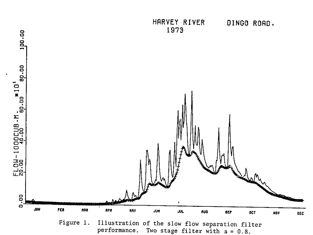
When modeling watershed hydrological processes, we often attempting to quantify
- watershed inputs
- e.g., precipitation
- e.g., precipitation
- watershed outputs
- e.g., evapotranspiration, sublimation, runoff/discharge
- e.g., evapotranspiration, sublimation, runoff/discharge
- watershed storage
- precipitation that is not immediately converted to runoff or ET rather stored as snow or subsurface water.
- precipitation that is not immediately converted to runoff or ET rather stored as snow or subsurface water.
Imagine we are trying to predict the percentage of precipitation stored in a watershed after a storm event. We have learned that there are may factors that affect this prediction, like antecedent conditions, that may be difficult to measure directly. Monte Carlo Simulation can offer a valuable approach to estimate the probability of obtaining certain measurements when those factors can not be directly observed or measured. We can approximate the likelihood of specific measurement by simulating a range of possible scenarios.
Monte Carlo Simulation is not only useful for estimating probabilities, but for conducting sensitivity analysis. In any model, there are usually several input parameters. Sensitivity analysis helps us understand how changes in these parameters affect the predicted values. To perform a sensitivity analysis using a Monte Carlo Simulation we can:
- Define the realistic ranges for each parameter we want to analyze
- Using Monte Carlo Simulation, randomly sample values from the defined ranges for each parameter
- Analyze output to understand how different input sample values affect the predicted output
2.5.1.4 Example
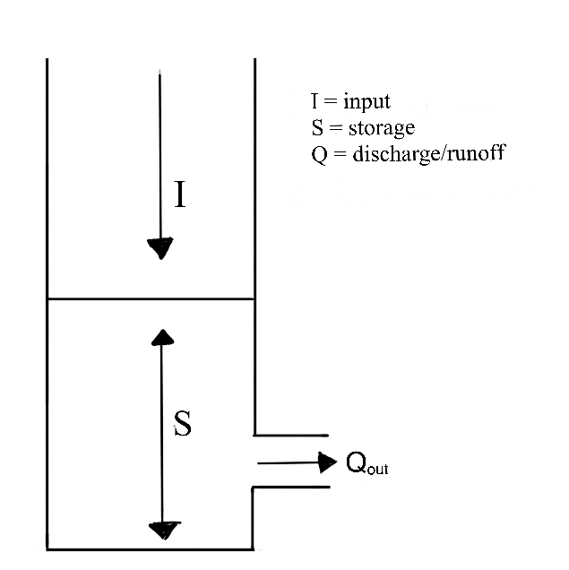
Let’s consider all of this in an example model called WECOH - Watershed ECOHydrology. In this study, researchers (Nippgen et al.) were interested in the change in subsurface water storage through time and space on a daily and seasonal basis.
The authors directly measured runoff/discharge, collected precipitation data at several points within the watershed, used remote sensing to estimate how much water was lost to evapotranspiration, and used digital elevation models to characterize the watershed topography. As we learned in the hydrograph separation module, topographic characteristics can have a significant impact on storage.
Though resources like USDA’s Web Soil Survey can provide a basic understanding underlying geology across a large region, characterizing the heterogeneous nature of soils within a watershed can be logistically unfeasible. To estimate the soil characteristics like storage capacity (how much water the soil can hold) and hydraulic conductivity (how easily water can move through soil) in the study watershed, the authors used available resources to determine the possible range of values for each of their unknown parameters. They then tested thousands of model simulations using randomly selected values with the predetermined range for each of the soil characteristics. They compared the simulated discharge from these simulations to the actual discharge measurements. The simulations that predicted discharge patterns that closely matched reality helped them to estimate the unknown soil properties. Additionally, from the results of these simulations, they could identify which model inputs had the most significant impact on the discharge predictions, and how sensitive the output was to changes in each parameter. In this case, they determined that the model and system were most sensitive to precipitation. This type of sensitivity analysis can help us interpret the relative importance of different parameters and understand the overall sensitivity of the model or system. The study is linked for your reference but a thorough reading is not required.
2.5.1.5 Reading
However, do read this methods paper by Knighton et al. for an example of how Monte Carlo Simulation was used to estimate hydraulic conductivity in an urban system with varied land-cover.
2.5.1.6 Generate a simulation with code
For a 12-minute example in RStudio, check this out. If you are still learning the basics of R functionality, it may be helpful to code along with this video, pausing as needed. Note that this instruction is coding in an Rscript (after opening RStudio > File > New File > R Script), rather than an Rmarkdown that we use in this class.
2.5.2 Labwork (20 pnts)
2.5.2.1 Download the repo for this lab HERE
In this lab/homework, you will use the transfer function model from the previous module for some sensitivity analysis using Monte Carlo simulations. The code is mostly the same as last module with some small adjustments to save the parameters from each Monte Carlo run. As a reminder, in the Monte Carlo analysis, we will run the model x number of times, save the parameters and evaluate the fit after each run. After the completion of the MC runs, we will use the GLUE method to evaluate parameter sensitivity. There are three main objectives for this homework:
1) Set up the Monte Carlo analysis
2) Run the MC simulation for ONE of the years in the study period and perform a GLUE sensitivity analysis
3) Compare the different objective functions.
A lot of the code in this homework will be provided.
2.5.2.2 Setup
Import packages, including the “progress” and “tictoc” packages. These will allow us to time our loops and functions
Read data - this is the same PQ data we have worked with in previous modules.
Define variables
2.5.2.3 Parameter initialization
This chunk has two purposes. The first is to set up the number of iterations for the Monte Carlo simulation. The entire model code is essentially wrapped into the main MC for loop. Each iteration of that loop is one full model realization: loss function, TF, convolution, model fit assessment (objective function). For each model run (each MC iteration), we will save the model parameters and respective objective functions in a dataframe. This will be the main source for the GLUE sensitivity analysis at the end. The model parameters are sampled in the main model chunk, this is just the preallocation of the dataframe.
You will both run your own MC simulation, to set up the code, but will also receive a .Rdata file with 100,000 runs to give you more behavioral runs for the sensitivity analysis and uncertainty bounds. As a tip, while setting up the code, I would recommend setting the number of MC iterations to something low, for example 10 or maybe even 1. Once you have confirmed that your code works, crank up the number of iterations. Set it to 1000 to see how many behavioral runs you get. After that, load the file with the provided runs.
2.5.2.4 MC Model run
This is the main model chunk. The tic() and toc() statements measure the execution time for the whole chunk. There is also a progressbar in the chunk that3 will run in the console and inform you about the progress of the MC simulation. The loss function parameters are set in the loss function, the TF parameters in the loss function code. For each loop iteration, we will store the parameter values and the simulated discharge in the “param” dataframe. So, if we ran the MC simulation 100 times, we would end up with 100 parameter combinations and simulated discharges.
Q1 (2 pt) How are the loss function and TF parameters being sampled? That is, what is the underlying distribution and why did we choose it? (2-3 sentences)
ANSWER:
Extra point: What does the while loop do in the TF calculation? And why is it in there? (1-2 sentences)
ANSWER:
Save or load data
After setting up the MC simulation, we will actually use a pre-created dataset. Running the MC simulation tens of thousands of times will take multiple hours. For that reason, we will use an existing data set.
Best run
Now that we have the dataframe with all parameter combinations and all efficiencies, we can plot the best simulation and compare it to the observed discharge
2.5.2.5 Sensitivity analysis
We will use the GLUE methodology to assess parameter sensitivity. We will use GLUE for two things: 1) To assess parameter sensitivity, and 2) to create an envelope of model simulations. For the first step, we need to bring the data into shape so that we can plot dotty plots and density plots. We will use NSE for this. You want to plot each parameter in its own box. Look up facet_wrap() for how to do this! You want the axis scaling to be “free”.
Q2 (4 pts) Describe the sensitivity analysis with the three different plots. Are the parameters sensitive? Which ones are, which ones are not? Does this affect your “trust” in the model? (5-8 sentences)
ANSWER:
Q3 (4 pts) What are the differences between the dotty plots and the density plots? What are the differences between the two density plots? (2-3 sentences)
ANSWER:
Uncertainty bounds In this chunk, we will generate uncertainty bounds for the simulation. We will again only use the runs that we identified as behavioral.
Q4 (3 pts) Describe what the envelope actually is. Could we say we are dealing with confidence or prediction intervals? (2-3 sentences)
ANSWER:
Q5 (3 pts) If you inspect the individual model runs (in the Qruns df), you will notice that they all perform somewhat poorly when it comes to the initial baseflow. Why is that and what could you do to change this? (Note: you don’t have to actually do this, just describe how you might approach that issue (2-3 sentences)
ANSWER:
Q6 (4 pts) Plot AND compare the best model run for the four objective functions. Note: This requires you to completely examine the figure generated in the previous code chunk. Remember that you can zoom into the plot to better see differences in peakflow and baseflow, timing, etc.(4+ sentences)
ANSWER:
The coding steps are: 1) get the simulated q vector with the best run for each objective function, 2) put them in a dataframe/tibble, 3) create the long form, 4) plot the long form dataframe/tibble. These steps are just ONE possible outline how the coding steps can be broken up.
Response surface