Chapter 5 DEM processing

5.1 THE LINK TO THE REPO IS HERE

15pnts

5.2 Objective:

Users will explore basic hydrological tools through the process of DEM preprocessing and defining stream networks for a watershed in the Fraser Experimental Forest in Colorado using Whitebox Tools for R. This exercise will also demonstrate methods for writing functions and efficiently handling multiple files simultaneously, including importing, processing, and exporting data within the context of Whitebox Tools for R.

5.3 Background:

Hydrological analysis preprocessing involves the use of digital elevation model (DEM) raster data to establish a watershed model and a simulation of surface hydrological processes. These steps enable us to quantify key parameters such as flow accumulation, stream network characteristics, and hydrological connectivity, which are essential for studying the dynamics of water movement within a landscape. Overall, preprocessing is the set of foundational steps in hydrological modeling and analysis.

Whitebox Tools is an advanced geospatial data analysis platform that can be used to perform common geographical information systems (GIS) analysis operations. This platform was developed with the Center for Hydrogeomatics in Guelph University so it is focused on hydrological analysis. With just a DEM, it allows us to produce a multitude of outputs that can be used for future analysis (Lindsay, 2016) doi:10.1016/j.cageo.2016.07.003). While we are demonstrating its use in R, these tools are also available in QGIS and Python platforms.

5.4 Codework

5.4.1 Installing libraries

We are going to try installing the whitebox R package from CRAN as it should be the simplest method.

However, if this does not work for you, you can install the development version from GitHub by putting this inside a code chunk:

if (!require(“remotes”)) install.packages(‘remotes’) remotes::install_github(“opengeos/whiteboxR”, build = FALSE)

More information on installation can be found at: https://cran.r-project.org/web/packages/whitebox/readme/README.html

Helpful whitebox documentation can be found at https://jblindsay.github.io/wbt_book/preface.html. Essentially, we will be using input rasters via filepath and output filepaths as arguments for various whitebox functions. The script is designed to perform functions on all rasters in a given folder at once.

When writing scripts, developers typically follow a standard workflow:
1. Import required libraries
2. Generate functions useful throughout the script
3. Establish working directories or paths to other directories if needed
4. Import data
5. Data Cleaning and Preprocessing - this may involve handling missing values, removing outlines, converting to preferred units. etc.
6. Exploratory Data Analysis - it is beneficial to explore data visually to help uunderstand the characteristics of the data.
7. Apply functions, or models or other analytical techniques
8. Evaluate results - If modeling, this may involve comparing model predictions with observed data or conducting sensitivity analysis
9. Visualize and report - plots, maps and tables can be effective ways to communicate findings.

While you might find slight variations among collaborators, following this general workflow ensures that our scripts are structured in a way that facilitates easy sharing and reproducibility of results.

5.4.2 Generate functions

Since we have imported the required libraries, let’s generate some functions.

# # extractsitename will extract a site name from the filepaths we provide. You will likely need to change the indexing in this function based on the filepaths to your DEMs. 
# extractsitename <- function(x) {
#     splitpath <- strsplit(x,'/')
#     basename <- splitpath[[1]][3]
#     splitbase <- strsplit(basename,'_')[[1]][1]
#     return(splitbase)
# }
# 
# #One method to determine how to assign correct indexes is to run each of the lines in this function in your console and view the results. For example, let's first list all files in your current working directory:
# 
# # List all files recursively in the current working directory
# all_files <- list.files(recursive = TRUE)

Q1.(2 pnt) What does date: “08 January, 2025” in the header do?

ANSWER:

Q2.(2 pnt) What does ‘recursive = TRUE’ do? What would the ‘recursive = FALSE’ return? ANSWER:

# # Now look at all_files printed in your console and select a filepath that represents a DEM. You can access that filepath alone by indexing all_files
# 
# print(all_files[3]) # you will likely have to change '3' here to match your filepath of choice

# # You can use this indexed file list to test each line of the extractsitename function to see what it does:
# splitpath <- strsplit(all_files[3], split = '/') # again, change '3' to match your filepath
# splitpath
# 
# # Note that strsplit splits a character string by whatever symbol or character we provide in the 'split' argument. Also note that splitpath is a list within a list, indicated by the double set of brackets around 1: [[1]]. We can 'unlist' splitpath, or we can call the string we want by using both list indexes:
# 
# basename <- splitpath[[1]][2] # here, basename should return the .tif name. If it does not, change the indices (likely '2') until your basename is the name of the tif. e.g., 'lexen_0.5m_DEM.tif'
# basename

# # Now we can split the tif name to extract the site name:
# splitbase <- strsplit(basename,'_')[[1]][1]
# splitbase

# Note that here we combined a couple of steps, splitting the file name and extracting the desired string in one line. 

# # Now let's save the function extractsitename again, but with the indices generate the sitenames using your current working directory.
# 
# extractsitename <- function(x) {
#     splitpath <- strsplit(x,'/')
#     basename <- splitpath[[1]][2]
#     splitbase <- strsplit(basename,'_')[[1]][1]
#     return(splitbase)
# }

# You can test the function in your console with: extractsitename(all_files[2]). This should return a site name (in this exercise, fool, lexen or deadhorse). 

EXTRA (1pnt) : Rewrite this function to generate ‘splitbase’ with fewer lines. For example, what happens when you replace ‘basename’ in ‘splitbase <- strsplit(basename,’_‘)[[1]][1]’ with ‘splitpath[[1]][2]’?

# Here we will generate another function that we will use later in the script. 
# 
# # Create a function to resample and export a single raster
# resample_and_export <- function(file_path) {
#   sitename <- extractsitename(file_path)
#   r <- raster(file_path) # Read in the raster
#   r_resamp <- aggregate(r, fact = 20) # Resample the raster
#   output_file_path <- file.path(paste0('resampleddems/', sitename, "_resampled.tif")) # Create the output file path
#   writeRaster(r_resamp, filename = output_file_path, format = "GTiff", overwrite = TRUE) # Export the resampled raster
#   return(list(sitename = sitename, output_file_path = output_file_path)) # Return the sitename and output file path as a list
# }

Q3. (2pnt) What is the point of writing a function and why do you think it is advantageous to write functions early in your script? ANSWER:

5.4.3 Establish new directories(folders)

in our working directory. We will use these to store the outputs of the Whitebox functions.

# # Define the directory names
# directory_names <- c('breachsinglecellpits', 'breachdep', 'resampleddems', 'd8pointer', 'logd8flowaccum', 'd8flowaccum', 'streams_wws','streams')
# 
# # Loop through each directory name
# for (dir_name in directory_names) {
#   # Check if the directory already exists, and create it if not
#   if (!dir.exists(dir_name)) {
#     dir.create(dir_name)
#   }
# }

Check your working directory, you should see the new folders there.

5.4.4 Resample DEMs

Here we will start with LiDAR data with 0.5m resolution. While this resolution has useful applications, a high resolution DEM can make hydrological models very computationally expensive with little or no improvement to the output. If you have the option of high resolution data in your work, you can test model outputs at different resolutions to determine what is the most efficient and effective resolution for your work. Here, we will resample our LiDAR data to a 10m resolution.

# # Resample dem to 10m
# 
# #List all of the dem files within the LiDARdem directory
# files <- list.files(path ='LiDARdem', pattern="*.tif", full.names=TRUE, recursive=FALSE)
# 
# # Use lapply to resample and export all resampled rasters
# output_files <- lapply(files, resample_and_export)

Q4. (3pnts) Did we use the function extractsitenames in the above chunk? How? What did it do?

ANSWER:

Let’s quickly check our work by importing a resampled DEM and checking the resolution.

# # Specify the path to the raster file
# path <- 'resampleddems/fool_resampled.tif'
# 
# # Import the raster
# raster_obj <- raster(path)
# 
# # Get the resolution
# resolution <- res(raster_obj)
# 
# # Print the resolution
# print(resolution)

Note: This can also be done without importing the raster to the workspace by installing the library gdalUtils.

Q5.(2pnts) What is the resolution of the resampled DEM? Where and how could we change the resolution to 30m if desired?

ANSWER:

# #List all of the resampled dem files within the resampleddems directory
# files <- list.files(path = paste('resampleddems', sep = "/"), pattern="*.tif", full.names=TRUE, recursive=FALSE)

5.4.5 Filling and breaching

When performing hydrological analysis on a DEM, the DEM usually needs to be pre-processed by ‘filling’ or ‘breaching’ any depressions or sinks to create a hydraulically connected and filled DEM. There are several depression or pit filling options available in whitebox. Breach depressions can be a better option that just pit filling according to whitebox documentation, however, some users argue that this can smooth too much, resulting in an altered watershed delineation. It is prudent to investigate different DEM pre-processing methods and their resulting DEM. You can fill depressions directly, breach depressions and then fill them, applying breach or fill single cell pit before breach/fill depressions, and use the one that generates the most reasonable watershed delineation results. Here we are going to make extra sure our flowpaths are uninhibited by first filling in single cell pits, and then breaching any larger depressions.

# #Fill single cell pits for all rasters the folder 'resampleddems' (for hydrologic correctness)
# 
# lapply(files, function(x) {
#     sitename <- extractsitename(x)
#     bscp <- wbt_breach_single_cell_pits(x, output = paste0(getwd(), '/breachsinglecellpits/', sitename, "_breach1")) #first wb function input
# })
# 
# #List all of the files from previous function 
# breach1 <- list.files(path= paste('breachsinglecellpits', sep = '/'), pattern="*.tif", full.names=TRUE, recursive=FALSE)
# 
# # apply breach depressions to every .tif in files list
# lapply(breach1, function(x) {
#     sitename <- extractsitename(x)
#     wbt_breach_depressions(x, output = paste0(getwd(),'/breachdep/', sitename, "_breachdep"), flat_increment=.01) #first wb function input
# })

5.4.6 Flow direction and accumulation rasters

# # List all of the filled files and use this list to make a flow direction grid and flow accumulation raster
# breachdep <- list.files(path = paste('breachdep', sep = "/"), pattern="*.tif", full.names=TRUE, recursive=FALSE)
# 
# #Flow direction grid (d8_pntr)
# lapply(breachdep, function(x) {
#     sitename <- extractsitename(x)
#     wbt_d8_pointer(x, output = paste0(getwd(), '/d8pointer/', sitename, "_d8pointer")) 
# })
# 
# # D8 flow accumulation (raster cells fully drain in 1 of 8 directions)
# 
# lapply(breachdep, function(x) {
#     sitename <- extractsitename(x)
#     wbt_d8_flow_accumulation(x, output = paste0(getwd(), '/logd8flowaccum/', sitename, "_logd8flowaccum"), 
#                              out_type='catchment area',
#                              log=T) 
# })
# 
# # Not log-transformed so output is the upslope accumulated area to each pixel in m2
# lapply(breachdep, function(x) {
#     sitename <- extractsitename(x)
#     wbt_d8_flow_accumulation(x, output = paste0(getwd(), '/d8flowaccum/', sitename, "_d8flowaccum"),
#                      out_type='catchment area',
#                      log=F)                              
# })

Q6 (2pnts) Check out the WhiteboxTools User Manual. What does a d8pointer raster tell us and what might we use it for? ANSWER:

Let’s visualize some of our work so far:

# #%%%%%%$$$$$$$$$ Visualize
# path <- paste0(getwd(), '/d8pointer/fool_d8pointer.tif')
# 
# checkwrk <- raster(path)
# mapview(checkwrk)

# #%%%%%%$$$$$$$$$ Visualize
# path <- paste0(getwd(), '/d8flowaccum/fool_d8flowaccum.tif')
# 
# checkwrk <- raster(path)
# mapview(checkwrk)

Q7. (2pnts) What are the units for the values that you see in each of these legends? It may be helpful to check out the Manual again. ANSWER:

5.4.7 Streams

Define streams using the flow accumulation raster. Use of the wbt_extract_streams function will return a raster with stream cells indicated only.

# #List all of the filled files 
# log_d8_flow_accum <- list.files(path = paste('logd8flowaccum', sep = "/"), pattern="*.tif", full.names=TRUE, recursive=FALSE)
# 
# lapply(log_d8_flow_accum, function(x) {
#   sitename <- extractsitename(x)
#   stream_raster <- wbt_extract_streams(x, output = paste0(getwd(), '/streams/', sitename, "_streams"), threshold = 12)
# })

# #%%%%%%$$$$$$$$$ Visualize
# path <- paste0(getwd(), '/streams/fool_streams.tif')
# 
# mapview(raster(path))

Sometimes we would prefer to see the stream within the watershed boundary. Here we are using the extent of the flow accumulation raster to generate a raster with ‘0’ to indicate watershed cells, along with stream cells indicated by the streams.tif. This is a demonstration for one watershed.

# input_path <- paste0(getwd(), '/streams/fool_streams.tif')
# # Read the output raster
# stream_raster <- raster(input_path)
#   
# # Convert NA to 0
# stream_raster[is.na(stream_raster)] <- 0
# 
# # Convert all non-zero values to 1
# stream_raster[stream_raster != 0] <- 1
# 
# # Create a zero raster with the same extent and resolution as the dem
# zero_raster <- raster(log_d8_flow_accum[2])
# zero_raster[is.na(log_d8_flow_accum[2])] <- NA
# zero_raster[!is.na(zero_raster)] <- 0
# 
# # Set the values in zero_raster to 1 where the stream_raster has 1
# zero_raster[stream_raster > 0] <- 1
# 
# # Write the final raster to file
# output_file_path <- file.path(getwd(), "streams_wws", paste0("fool_streams_wws.tif"))
# writeRaster(zero_raster, filename = output_file_path, format = "GTiff", overwrite = TRUE)

# #%%%%%%$$$$$$$$$ Visualize
# path <- paste0(getwd(), '/streams_wws/fool_streams_wws.tif')
# 
# mapview(raster(path))

5.4.8 Final thoughts:

There are many more hydrological preprocessing and analysis tools available through Whitebox for R. If you are interested in watershed delineation in R, there is a tutorial here that is fairly easy to follow. However, if you find that you use these tools frequently and do not use R much in other work, you may also consider these options for hydrological analysis:

1. SAGA SAGA tools offer a versatile suite of geospatial processing capabilities accessible through both QGIS and ArcGIS plugins as well their standalone GUI interface. Often I find the GUI easiest for preprocessing, then I will import SAGA’s output rasters to QGIS for formatting or map making, or into model scripts. SAGA has a robust online support community, so it can be a valuable resource for hydrological work.

2. Similarly, Whitebox GAT tools can be used as plugin to QGIS and ArcGIS, providing Whitebox functionality directly with in a GIS environment.
When using these tools, the order of operations is similar to our work above: fill the DEM, generate a flow direction and flow accumulation raster, identify channels, delineate watersheds, then you can move forward according to the specificity of your project. Ultimately, the choice of workflow is yours, but I suggest documenting your process as you proceed, including links or file paths to projects and scripts within the written workflow. It’s also important to carefully consider the organization and storage of your projects and files. For instance, files generated by a GIS project should be readily accessible to any associated scripts. Returning to a preprocessing step can be challenging if there’s no clear way to trace back your workflow and regenerate a crucial layer.

5.5 Transfer function rainfall-runoff models

5.5.1 Summary

In previous modules, we explored how watershed characteristics influence the flow of input water through or over hillslopes to quickly contribute to stormflow or to be stored for later contribution to baseflow. Therefore, the partitioning of flow into baseflow or stormflow can be determined by the time it spends in the watershed. Furthermore, the residence time of water in various pathways may affect weathering and solute transport within watersheds. To improve our understanding of water movement within a watershed, it can be crucial to incorporate water transit time into hydrological models. This consideration allows for a more realistic representation of how water moves through various storage compartments, such as soil, groundwater, and surface water, accounting for the time it takes for water to traverse these pathways.

In this module, we will model the temporal aspects of runoff response to input using a transfer function. First, please read:

TRANSEP - a combined tracer and runoff transfer function hydrograph separation model

Then this chapter will step through key concepts in the paper to facilitate hands-on exploration of the rainfall-runoff portion of the TRANSEP model in the assessment. Then, we will introduce examples of other transfer functions to demonstrate alternative ways of representing time-induced patterns in hydrological modeling, prompting you to consider response patterns in your study systems.

5.5.2 Overall Learning Objectives

At the end of this module, students should be able to describe several ways to model and identify transit time within hydrological models. They should have a general understanding of how water transit time may influence the timing and composition of runoff.

5.5.3 Terminology

In modeling a flow system, note that consideration of time may vary depending on the questions being asked. Transit time is the average time required for water to travel through the entire flow system, from input (e.g., rainfall on soil surface) to output (e.g., discharge). Residence time is a portion of transit time, describing the amount of time water spends within a specific component of the flow system, like storage (e.g., in soil, groundwater, or a lake).

Figure 6.3. Conceptual diagram of the lumped parameter transit time modeling approach (McGuire & McDonnell, 2006)

A transfer function (TF) is a mathematical representation of how a system responds to input signals. In a hydrological context, it describes the transformation of inputs (e.g. precipitation) to outputs (e.g. runoff). These models can be valuable tools for understanding the time-varying dynamics of a hydrological system.

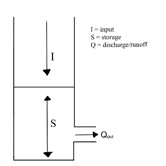
5.5.4 The Linear Time-Invariant TF

We’ll begin the discussion in the context of a linear reservoir. Linear reservoirs are simple models designed to simulate the storage and discharge of water in a catchment. These models assume that the catchment can be represented as single storage compartments or as a series of interconnected storage compartments and that the change the amount of water stored in the reservoir (or reservoirs) is directly proportional to the inflows and outflows. In other words, the linear relationship between inflows and outflows means that the rate of water release is proportional to the amount of water stored in the reservoir.

5.5.4.0.1 The Instantaneous Unit Hydrograph:

The Instantaneous Unit Hydrograph (IUH) represents the linear rainfall-runoff model used in the TRANSEP model. It is an approach to hydrograph separation that is useful for analyzing the temporal distribution of runoff in response to a ‘unit’ pulse of rainfall (e.g. uniform one-inch depth over a unit area represented by a unit hydrograph). In other words, it is a hydrograph that results from one unit (e.g. 1 mm) of effective rainfall uniformly distributed over the watershed and occurring in a short duration. Therefore, the following assumptions are made when the IUH is used as a transfer function:
1. the IUH reflects the ensemble of watershed characteristics
2. the shape characteristics of the unit hydrograph are independent of time
3. the output response is linearly proportional to the input

Figure 6.4.1.a Conceptual diagram of the linear unit hydrograph

Peak discharge of the unit hydrograph, \(u_p\);
Base time \(t_b\)is the total duration of the unit hydrograph;
Increase time or time to peak \(t_p\) is the time between the start point of the hydrograph and the peak;
Concentration time \(t_c\) is the time between the end of rainfall and the end of the hydrograph;
Lag time \(t_lag\) is the time between half rainfall depth and the peak of the hydrograph.

IUH as a transfer function allows the calculation of the direct runoff hydrograph for any given rainfall input. IUH is particularly valuable for understanding how the direct runoff is distributed over time in response to a rainfall event. It helps quantify the time distribution of runoff in relation to the rainfall input.

Figure 6.4.1.b The discharge of the unit hydrograph(u) from a catchment at time (t) is expressed as \(h \cdot u(t)\) where h is the amount of effective rainfall.

In the TRANSEP model, this transfer function is represented as \(g(\tau)\) and thus the rainfall-induced response to runoff.

\[ g(\tau) = \frac{\tau^{\alpha-1}}{\mathrm{B}^{\alpha}\Gamma(\alpha)}exp(-\frac{\tau}{\alpha}) \]

The linear portion of the TRANSEP model describes a convolution of the effective precipitation and a runoff transfer function.

\[ Q(t)= \int_{0}^{t} g(\tau)p_{\text{eff}}(t-\tau)d\tau \]

Whoa, wait…what? Tau, integrals, and convolution? Don’t worry about the details of the equations. Check out this video to have convolution described using dollars and cookies, then imagine each dollar as a rainfall unit and each cookie as a runoff unit. Review the equations again after the video.

knitr::include_url("https://www.youtube.com/embed/aEGboJxmq-w")

5.5.4.0.2 The Loss Function:

The loss function represents the linear rainfall-runoff model used in the TRANSEP model.

\[ s(t) = b_{1} p(t + 1 - b_{2}^{-1}) s(t - \triangle t) \] \[ s(t = 0) = b_{3} \] \[ p_{\text{eff}}(t) = p(t) s(t) \] where \(p_{\text{eff}}(t)\) is the effective precipitation.
\(s(t)\) is the antecedent precipitation index which is determined by giving more importance to recent precipitation and gradually reducing that importance as we go back in time.
The rate at which this importance decreases is controlled by the parameter \(b_{2}\).
The parameter \(b_{3}\) sets the initial antecedent precipitation index at the beginning of the simulated time series.

In other words, these equations are used to simulate the flow of water in a hydrological system over time. The first equation represents the change in stored water at each time step, taking into account precipitation, loss to runoff, and the system’s past state. The second equation sets the initial condition for the storage at the beginning of the simulation. The third equation calculates the effective precipitation, considering both precipitation and the current storage state.

5.5.4.0.3 How do we code this?

We will use a skeletal version of TRANSEP, focusing only on the rainfall-runoff piece which includes the loss-function and the gamma transfer function.

We will use rainfall and runoff data from TCEF to model annual streamflow at a daily time step. Then we can use this model as a jump-off point to start talking about model calibration and validation in future modules.

5.5.4.0.4 Final thoughts:

If during your modeling experience, you find yourself wading through a bog of complex physics and multiple layers of transfer functions to account for every drop of input into a system, it is time to revisit your objectives. Remember that a model is always ‘wrong’. Like a map, it provides a simplified representation of reality. It may not be entirely accurate, but it serves a valuable purpose. Models help us understand complex systems, make predictions, and gain insights even if they are not an exact replica of the real world. Check out this paper for more:

https://agupubs.onlinelibrary.wiley.com/doi/10.1029/93WR00877

5.5.5 Labwork (20 pts)

5.5.5.1 Download the repo for this lab HERE

In this homework/lab, you will write a simple, lumped rainfall-runoff model. The foundation for this model is the TRANSEP model from Weiler et al., 2003. Since TRANSEP (tracer transfer function hydrograph separation model) contains a tracer module that we don’t need, we will only use the loss function (Jakeman and Hornberger) and the gamma transfer function for the water routing.
The data for the model is from the Tenderfoot Creek Experimental Forest in central Montana.

Load packages with a function that checks and installs packages if needed:

#knitr::opts_chunk$set(echo = FALSE)

# 
# # Write your package testing function
# pkgTest <- function(x)
# {
#   if (x %in% rownames(installed.packages()) == FALSE) {
#     install.packages(x, dependencies= TRUE)
#   }
#   library(x, character.only = TRUE)
# }
# 
# # Make a vector of the packages you need
# neededPackages <- c('tidyverse', 'lubridate', 'tictoc', 'patchwork') #tools for plot titles 
# 
# # For every package in the vector, apply your pkgTest function
# for (package in neededPackages){pkgTest(package)}
# 
# # tictoc times the execution of different modeling methods
# # patchwork is used for side-by-side plots

# # Let's assume that you know you put your data file in the working directory, but cannot recall its name. Let's do some working directory exploration with script:
# 
# # Check your working directory:
# print(getwd())
# 
# # Check the datafile name or path by listing files in the working directory.
# filepaths <-list.files()
# 
# # Here is an option to list only .csv files in your working directory:
# csv_files <- filepaths[grepl(".csv$", filepaths, ignore.case = TRUE)]
# print(csv_files)
# ```
# 
# #### Read in the data, convert the column that has the date to a (lubridate) date, and add a column that contains the water year

# # Identify the path to the desired data. 
# filepath <- "P_Q_1996_2011.csv"
# indata <- read.csv(filepath)
# 
# indata <- indata %>%
#   mutate(Date = mdy(Date)) %>% # convert "Date" to a date object with mdy()
#   mutate(wtr_yr = if_else(month(Date) > 9, year(Date) + 1, year(Date)))

Define input year We could use every year in the time series, but for starters, we’ll use 2006. Use filter() to extract the 2006 water year.

# PQ <- indata %>%
#   filter(wtr_yr == 2006) # extract the 2006 water year with filter()
# 
# # plot discharge for 2006
# ggplot(PQ, aes(x = Date, y = Discharge_mm)) +
#   geom_line()
# 
# # make flowtime correction - flowtime is a time-weighted cumulative flow, which aids in understanding the temporal distribution of flow, giving more weight to periods of higher discharge. flow time correction is relevant in hydrology when analyzing Q or time series data, so we can compare hydrological events on a standardized time scale. It can help to identify patterns, assess the duration of high or low flows, and compare behavior of watersheds over time.
# 
# PQ <- PQ %>% 
#   mutate(flowtime = cumsum(Discharge_mm)/mean(Discharge_mm)) %>% 
#   mutate(counter = 1:nrow(PQ))
# 
# ggplot() +
#   geom_line(data=PQ, aes(x = flowtime, y = Discharge_mm)) + 
#   geom_line(data=PQ, aes(x = counter, y = Discharge_mm), color="red")

1) QUESTION: What does the function cumsum() do?(1 pt) ANSWER:

Define the initial inputs

This chunk defines the initial inputs for measured precip and measured runoff

# tau <- 1:nrow(PQ) # simple timestep counter the same length as PQ
# Pobs <- PQ$RainMelt_mm # observed precipitation from PQ df
# Qobs <- PQ$Discharge_mm # observed streamflow from PQ df

Parameterization

We will use these parameters. You can change them if you want, but I’d suggest leaving them like this at least until you get the model to work. Even tiny changes can have a huge effect on the simulated runoff.

# # Loss function parameters
# b1 <- 0.0018 # volume control parameter (b1 in eq 4a)
# b2 <- 50 # backwards weighting parameter (b2 in eq 4a) 
# # determines how much weight or importance is given to past precipitation events when calculating an antecedent precipitation index. "Exponential weighting backward in time" means that the influence of past precipitation events diminishes as you move further back in time, and this diminishing effect follows an exponential pattern.
# 
# b3 <- 0.135 # initial s(t) value for s(t=0) (b3 in eq 4b) - Initial antecedent precipitation index value.
# 
# # Transfer function parameters
# a <- 1.84 # TF shape parameter
# b <- 3.29 # TF scale parameter

Loss function

This is the module for the Jakeman and Hornberger loss function where we turn our measured input precip into effective precipitation (p_eff). This part contains three steps.
1) preallocate a vector p_eff: Initiate an empty vector for effective precipitation that we will fill in with a loop using Peff(t) = p(t)s(t). Effective precipitation is the portion of precipitation that generates streamflow and event water contribution to the stream. It is separated to produce event water and displace pre-event water into the stream. 2) set the initial value for s: s(t) is an antecedent precipitation index. How much does antecedent precipitation affect effective precipitation? 3) generate p_eff inside of a for-loop
Please note: The Weiler et al. (2003) paper states that one of the loss function parameters (vol_c) can be determined from the measured input. That is actually not the case.

s(t) is the antecedent precipitation index that is calculated by exponentially weighting the precipitation backward in time according to the parameter b2 is a ‘dial’ that places weight on past precipitation events.

# # preallocate the p_eff vector
# p_eff <- vector(mode = "double", length(tau))
# 
# s <- b3 # at this point, s is equal to b3, the start value of s
# 
# # loop with loss function
# for (i in 1:length(p_eff)) {
#   s <- b1 * Pobs[i] + (1 - 1/b2) * s # this is eq 4a from Weiler et al. (2003)
#   p_eff[i] <- Pobs[i] * s # this is eq 4c from Weiler et al. (2003)
# }
# 
# 
# # #### alternative way to calculate p_eff by populating an s vector  
# # preallocate s_alt vector
# # s_alt <- vector(mode = "double", length(tau))
# # s_alt[1] <- b3
# # # preallocate p_eff vector
# # p_eff_new <- vector(mode = "double", length(tau))
# # # start loop
# # for (i in 2:(length(p_eff))) {
# #   s_alt[i] <- b1 * Pobs[i] + (1 - 1/b2) * s_alt[i-1]
# #   p_eff_new[i] <- Pobs[i] * s_alt[i]
# # }
# ####
# # set a starting value for s
# 
# 
# ## plot observed and effective precipitation against the date
# # wide to long with pivot_longer()
# precip <- tibble(date = PQ$Date, obs = Pobs, sim = p_eff) %>%
#   pivot_longer(names_to = "key", values_to = "value", -date)
# 
# 
# # a good way to plot P time series is with a step function. ggplot2 has geom_step() for this.
# ggplot(precip, aes(x = date, y = value, color = key)) +
#   geom_step() +
#   labs(color = "P")
# 
# 
# ## plot the ratio of p_eff/Pobs (call that ratio "frac")
# precip_new <- tibble(date = PQ$Date, obs = Pobs, sim = p_eff, frac = p_eff/Pobs)
# 
# ggplot(data = precip_new, aes(x = date, y = frac)) +
#   geom_line()

2) QUESTION (3 pts): Interpret the two figures. What is the meaning of “frac”? For this answer, think about what the effective precipitation represents. When is frac “high”, when is “frac” low?

ANSWER:

Extra Credit (2 pt): Combine the two plots into one, with a meaningfully scaled secondary y-axis

Runoff transfer function

Routing module -

This short chunk sets up the TF used for the water routing. This part contains only two steps: 1) the calculation of the actual TF. 2) normalization of the TF so that the sum of the TF equals 1.

tau(0) is the mean residence time

# #gTF <- tau
# 
# # this is the "raw" transfer function. This is eq 13 from Weiler 2003. Use the time step for tau. The Gamma function in R is gamma(). NOTE THAT THIS EQ IN WEILER ET AL IS WRONG! It's exp(-tau / b) and not divided by alpha.
# g <- (tau^(a - 1)) / ((b^a * gamma(a))) * exp(-tau / b)
# 
# # normalize the TF, g, by the total sum of g.
# gTF <- g / sum(g)
# 
# # plot the TF as a line against tau. You need to put the two vectors tau and gTF into a new df/tibble for this. 
# tf_plot <- tibble(tau, gTF)
# ggplot(tf_plot, aes(tau, gTF)) +
#   geom_line()

3) QUESTION (2 pt): Why is it important to normalize the transfer function?
ANSWER:

4) QUESTION (4 pt): Describe the transfer function. What are the units and what does the shape of the transfer function mean for runoff generation?
ANSWER:

Convolution

This is the heart of the model. Here, we convolute the input with the TF to generate runoff. There is another thing you need to pay attention to: We are only interested in one year (365 days), but since our TF itself is 365 timesteps long, small parts of all inputs except for the first one, will be turned into streamflow AFTER the water year of interest, that is, in the following year. In practice, this means you have two options to handle this.
1) You calculate q_all and then manually cut the matrix/vector to the correct length at the end, or
2) You only populate a vector at each time step and put the generated runoff per iteration in the correct locations within the vector. For this to work, you would need to trim the length of the generated runoff by one during each iteration. This approach is more difficult to code, but saves a lot of memory since you are only calculating/storing one vector of length 365 (or 366 during a leapyear).
We will go with option 1). The code for option 2 is shown at the end for reference.

Convolution summarized (recall dollars and cookies): Each loop iteration results in a row of the matrix representing the convolution at a specific time step. each time step of p_eff is an iteration, and for each timestep, it multiplies the effective precipitation at that timestep by the entire transfer function. Then each row is summed and stored in the vector q_all. q_all_loop is an intermediate step in the convolution process and can help visualize how the convolution evolves over time. As an example, if we have precip at time step 1, we are interested in how this contributes to runoff at time steps 1,2,3 etc, all the way to 365 (or the end of our period). so the first row of the matrix q_all_loop represents the contribution of precipitation at timestep 1 to runoff at each timestep. the second row represents the contribution of precipitation at time step 2 to runoff at each timestep. Then when we sum up the rows, we get q_all, where each element represents the total runoff at a specific time step.

# tic()
# # preallocate qsim matrix with the correct dimensions. Remember that p_eff and gTF are the same length.
# q_all_loop <- matrix(0, length(p_eff) * 2, length(p_eff)) # set number of rows and columns
# 
# # convolution for-loop
# for (i in 1:length(p_eff)) { # loop through length of precipitation timeseries
#   q_all_loop[(i):(length(p_eff) + i - 1), i] <- p_eff[i] * gTF # populate the q_all matrix (this is the same code as the UH convolution problem with one tiny change because you need to reference gTF and not UH)
# }
# 
# 
# # add up the rows of the matrix to generate the final runoff and replace matrix with final Q
# q_all <- apply(q_all_loop, 1, sum, na.rm = TRUE)
# 
# # cut the vector to the appropriate length of one year (otherwise it won't fit into the original df with the observed data)
# q_all <- q_all[1:length(p_eff)]
# 
# # Write the final runoff vector into the PQ df
# PQ$Qsim <- q_all
# toc()

5) QUESTION (5 pts): We set the TF length to 365. What is the physical meaning of this (i.e., how well does this represent a real system and why)? Could the transfer function be shorter or longer than that?

ANSWER:

# ## THIS PART SAVES ALL HOURLY Q RESPONSES IN A NEW DF AND PLOTS THEM
# Qall <- as_tibble(q_all_loop, .name_repair = NULL)
# Qall <- Qall[ -as.numeric(which(apply(Qall, 2, var) == 0))]
# toc()
# 
# # Qall[Qall == 0] <- NA
# 
# Qall <- Qall %>%
#   mutate(Time_hrs = 1:nrow(Qall)) %>% # add the time vector
#   gather(key, value, -Time_hrs)
# 
# Qall$key <- as.factor(Qall$key)
# 
# 
# ggplot(Qall, aes(x = Time_hrs, y = value, fill = key)) +
#   geom_line(alpha = 0.2) +
#   theme(legend.position = "none") +
#   lims(x = c(1, 365)) +
#   labs(x = "DoY", y = "Q (mm/day")

Plots

Plot the observed and simulated runoff. Include a legend and label the y-axis.

# # make long form
# PQ_long <- PQ %>%
#   select(-wtr_yr, -RainMelt_mm) %>%
#   pivot_longer(names_to = "key", values_to = "value", -Date)
# 
# # plot hydrographs (as lines) and label the y-axis
# ggplot(data = PQ_long, aes(x = Date, y = value, color = key)) +
#   geom_line() +
#   labs(x = {}, y = "Q (mm/day)", color = {}) +
#   lims(x = as.Date(c("2005-10-01", "2006-09-30")))

6) QUESTION (3 pt): Evaluate how good or bad the model performed (i.e., visually compare simulated and observed streamflow, e.g., low flows and peak flows).
ANSWER:

7) QUESTION (2 pt): Compare the effective precipitation total with the simulated runoff total and the observed runoff total. What is p_eff and how is it related to q_all? Discuss why there is a (small) mismatch between the sums of p_eff and q_all.
ANSWER:

# sum(Pobs) # observed P
# 
# sum(p_eff) # effective (modeled) P
# 
# sum(q_all) # modeled Q
# 
# sum(Qobs) # observed Q

THIS IS THE CODE FOR CONVOLUTION METHOD 2
This method saves storage requirements since only a vector is generated and not a full matrix that contains all response pulses. The workflow here is to generate a a response vector for the first pulse. This will take up 365 time steps. On the second time step, we generate another response pulse with 364 steps that starts at t=2. We then add that vector to the first one. On the third time step, we generate a response pulse of length 363 that starts at t=3 and then add it to the existing one. And so on and so forth.

# # METHOD 2, Option 1
# tic()
# # preallocate qsim vector
# q_all <- vector(mode = "double", length(p_eff))
# # start convolution
# for (i in 1:length(p_eff)) {
#   A <- p_eff[i] * gTF # vector with current Q pulse
#   B <- vector(mode = "double", length(p_eff)) # reset/preallocate vector with 0s
#   B[i:length(p_eff)] <- A[1:(length(p_eff) - i + 1)] # iteration one uses the full A, iteration 2 full lengthmodel minus one, etc
#   q_all <- q_all + B # add new convoluted vector to total runoff
# }
# toc()
# 
# 
# # Method 2, Option 2
# tic()
# # preallocate qsim vector
# q_all_2 <- vector(mode = "double", length(p_eff))
# B <- vector(mode = "double", length(p_eff)) # preallocate vector with 0s
# 
# # start convolution
# for (i in 1:length(p_eff)) {
#   A <- p_eff[i] * gTF # vector with current Q pulse
#   B[i:length(p_eff)] <- A[1:(length(p_eff) - i + 1)] # iteration one uses the full A, iteration 2 full lengthmodel minus one, etc
#   q_all_2[i:length(p_eff)] <- q_all_2[i:length(p_eff)] + B[i:length(p_eff)] # add new convoluted vector to total runoff at correct locations
# }
# toc()
# 
# # plot to show the two Q timeseries are the same
# # Create two ggplot objects
# plot_q1 <- ggplot(data=test_q_all, aes(x=time, y=q1)) +
#   geom_line() +
#   labs(title = "Q1 Plot")
# 
# plot_q2 <- ggplot(data=test_q_all, aes(x=time, y=q2)) +
#   geom_line(color="blue") +
#   labs(title = "Q2 Plot")
# 
# # Combine plots side by side
# combined_plots <- plot_q1 + plot_q2 + plot_layout(ncol = 2)
# 
# # Display combined plots
# combined_plots