Chapter 3 Fundamentals of Hydrological Analysis - Physical Hydrology and Empirical Methods
3.1 Hydrograph separation
- This module was developed by Ana Bergrstrom and Matt Ross.
3.1.1 Learning Module 1
3.1.1.1 Summary
Streamflow can come from a range of water sources. When it is not raining, streams are fed by the slow drainage of groundwater. When a rainstorm occurs, streamflow increases and water enters the stream more quickly. The rate at which water reaches the stream and the partitioning between groundwater and faster flow pathways is variable across watersheds. It is important to understand how water is partitioned between fast and slow pathways (baseflow and stormflow) and what controls this partitioning in order to better predict susceptibility to flooding and if and how groundwater can sustain streamflow in long periods of drought.
In this module we will introduce the components of streamflow during a rain event, and how event water moves through a hillslope to reach a stream. We will discuss methods for partitioning a hydrograph between baseflow (groundwater) and storm flow (event water). Finally, we will explore how characteristics of a watershed might lead to more or less water being partitioned into baseflow vs. stormflow. We will test understanding through evaluating data collected from watersheds in West Virginia to determine how mountaintop mining, which fundamentally changed the watershed structure, affects baseflow.
3.1.1.2 Reading for this lab
Ladson, A. R., R. Brown, B. Neal and R. Nathan (2013) A standard approach to baseflow separation using the Lyne and Hollick filter. Australian Journal of Water Resources 17(1): 173-18
Lynne, V., Hollick, M. (1979) Stochastic time-variable rainfall-runoff modelling. In: pp. 89-93 Institute of Engineers Australia National Conference. Perth.
3.1.1.3 Overall Learning Objectives
At the end of this module, students should be able to describe the components of streamflow, the basics of how water moves through a hillslope, and the watershed characteristics that affect partitioning between baseflow and stormflow.
3.1.1.5 Components of streamflow during a rain event
During a rainstorm, precipitation is falling across the watershed: close
to the stream, on a hillslope, and up at the watershed divide. This
water that falls across the watershed flows downslope toward the stream
via a number of flow pathways. Here we define and describe the basic
flow pathways during a rain event.
The first component is channel interception. This is water that
falls directly on the water surface of the stream. The amount of water
that falls directly on the channel is a function of stream size, if we
have a very small, narrow creek, this will be a very small quantity.
However, you can imagine that in a very large, broad river such as the
Amazon, this volume of water is much larger. Channel interception is the
first component during a rain event that causes streamflow to increase
because it is contributing directly to the stream and therefore has no
travel time.
The second is overland flow, which is water that flows on the land surface to the stream. Overland flow can occur via a number of mechanisms which we will not explore too deeply here, but encourage further study on your own (resources provided). Briefly, overland flow includes water that falls on an impermeable surface such as pavement, water that runs downslope due to rain falling faster than the rate at which it can infiltrate the ground surface, and water that flows over the land surface because the ground is completely saturated. Overland flow is typically faster than water that travels through soils and deeper flow pathways and therefore is the next major component that starts to contribute to the increase in streamflow during a rain event.
The third component is subsurface flow. This is water that infiltrates the land surface and flows downslope through shallow groundwater flow pathways. This is the last component that increases streamflow during a storm event, is the slowest of the stormflow components, and can contribute to elevated streamflow for a while after precipitation ends.
The final component is baseflow. Baseflow can also be described as groundwater. This component is what sustains streamflow between rain events, but also continues to contribute during a rain event. Of water that infiltrates the ground surface, some moves quickly to the stream as subsurface flow, but some moves deeper and becomes part of deeper groundwater and baseflow. Thus baseflow can increase in times of higher wetness in the watershed, particularly during and right after rainy seasons or spring snowmelt.
We can simplify this partitioning into baseflow and stormflow (often called quickflow). Baseflow being groundwater that moves more slowly and sustains streamflow between rain events. Stormflow is water that contributes to streamflow as a result of a rain event. Under this definition we can lump channel interception, overland flow, and subsurface flow into stormflow.
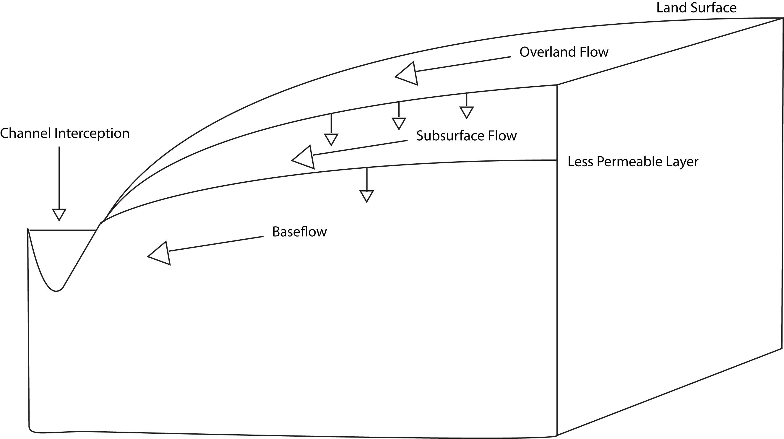
3.1.1.6 Storm flow through a hillslope
When rain falls on the land surface, much of it infiltrates into the soil. Water moves through the soil column until it meets a layer of lower permeability and runs down the hillslope as subsurface flow. This layer of lower permeability allows some water to move through it, contributing to groundwater. Frequently the layer of lower permeability is the interface between soil and rock. Therefore the depth of soil has a large effect on how much water moves through soil vs. how much moves deeper into groundwater, becoming baseflow.
3.1.1.7 How we quantify baseflow
It is impossible to know the amount of water moving as overland, subsurface, and base flow in all parts of a watershed. So in order to quantify how much water in a stream at any given time is storm flow vs. baseflow, we need to use some simplified methods (i.e., modeling). These frequently involve using the hydrograph (plot of streamflow over time) drawing lines, and calculating the volume of water above and below the line. This can be somewhat arbitrary and there are a variety of methods for delineating the cutoff between baseflow and stormflow. Despite what method you use and how simplified it is, this technique still provides valuable information and allows us to make comparisons across watersheds in order to understand how they function and what their structural properties are.
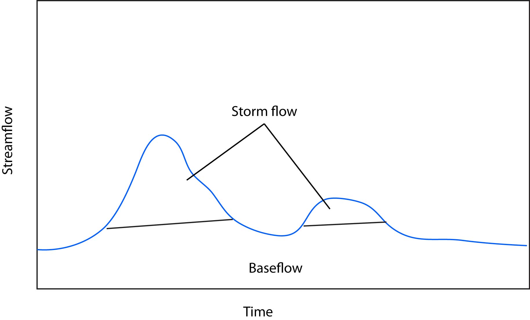
3.1.1.8 Baseflow separation methods
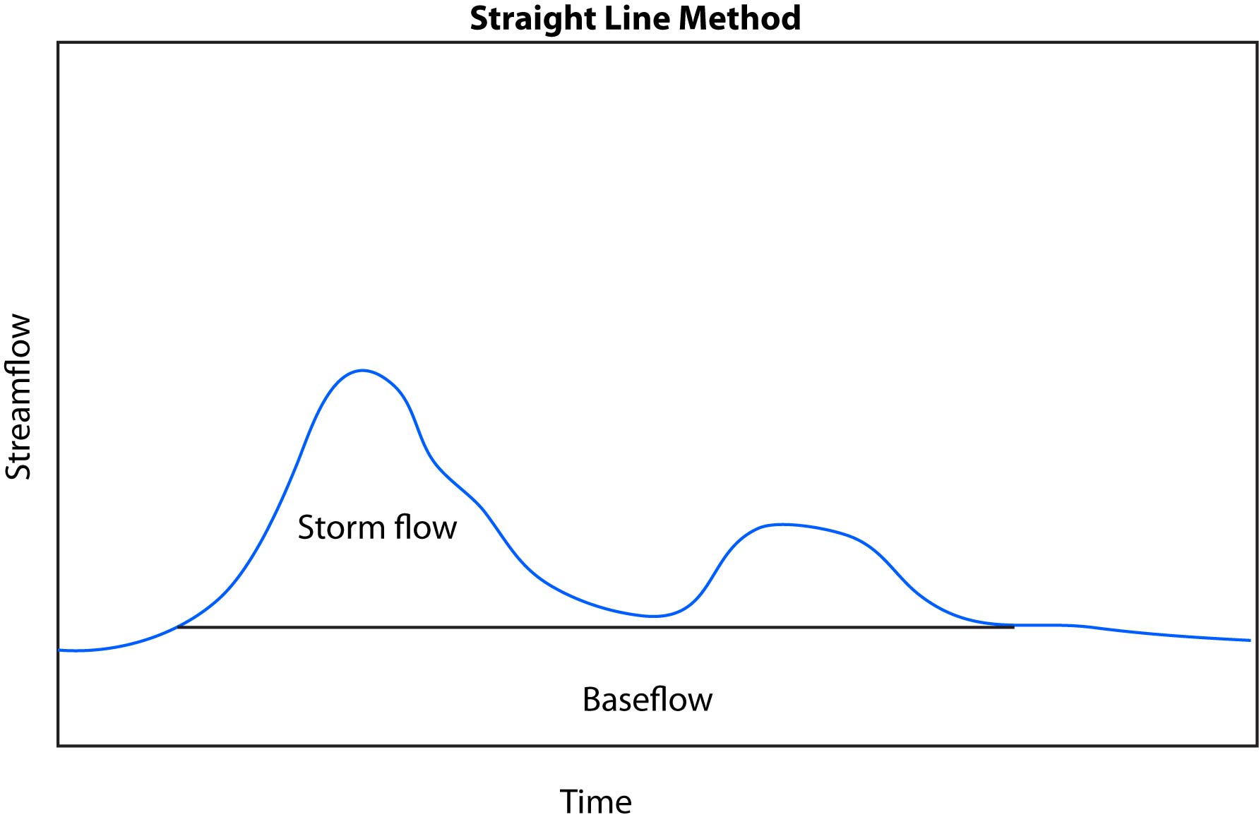
One of the most basic methods for calculating base flow vs. storm flow is the straight line method. First, find the value of discharge at the point that streamflow begins to rise due to a storm. A straight line is drawn at that value until it intersects with the hydrograph (i.e. streamflow recedes back to the discharge it was at before the rainfall event started. Anything below this line is base flow and anything above it is storm flow.
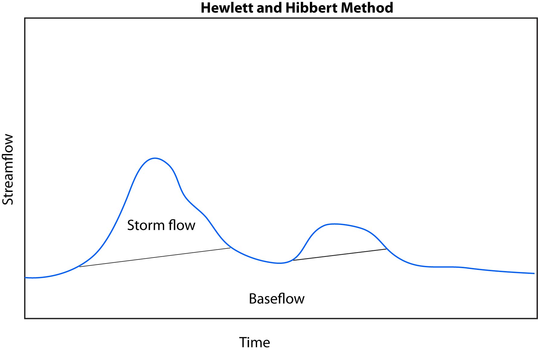
We learned above that some rainfall can move deep into the soil profile and contribute to baseflow. We might expect baseflow to increase over time and thus would want to use a method that can account for this.
An addition to the straight line method was posed by Hewlett and Hibbert, 1967. This method, which we’ll call the Hewlett and Hibbert method finds the discharge at the starting point of a storm. Then, rather than a straight line of 0 slope and in the straight line method, we assume a slope of 0.05 cubic feet per second per square mile. The line with this calculated slope is drawn until it intersects with the hydrograph receding at the end of the storm.
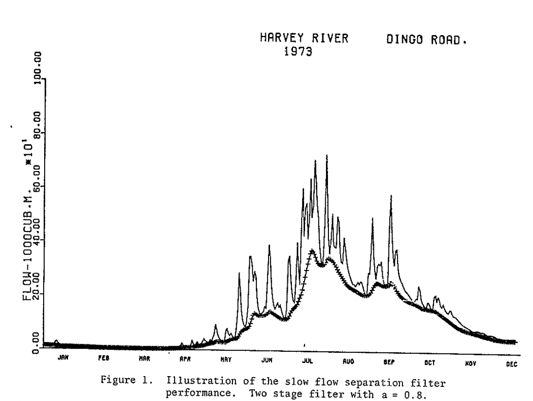
There are myriad other methods for baseflow separation of a wide range of complexity. We will give an example of one more method: a recursive filter method established by Lyne and Hollick (1976). This method smooths the hydrograph and partitions part of that smoothed signal into baseflow. The equation for this method is:
You can see from this equation that a filter parameter, a, must be chosen. This parameter can be decided by the user, takes a value between 0 and 1, and is typically close to 1. Additionally this filtering method must be constrained so that baseflow is not negative or greater than the total streamflow. Output from this method for the Harvey River in Australia is originally published in Lyne and Hollick (1976) below (notice in the caption that the a parameter was set to 0.8):
3.1.1.9 Watershed controls on baseflow and stormflow
The way a watershed is structured has a strong control on how water is
partitioned into baseflow and stormflow. Below is a list of key
structural properties: Land Use and Land Cover: If a watershed is
developed or natural can dictate how much water infiltrates the land
surface and how quickly. For example, a watershed with lots of pavement
means that much more water will be overland flow with fewer
opportunities to recharge baseflow. Furthermore, how a watershed is
developed will affect partitioning. For example a residential area with
houses on large, grassy lots will allow for more infiltration than a
shopping center with large parking lots. Land cover in natural areas
will also affect partitioning. Some other variables to consider may be:
Land cover in natural areas: a dense forest vs. a recently
harvested hillside.
Soil type: clayey soils vs. sandy soils
Depth to impeding layer: could be the bedrock interface, but could also
be a low permeability clay layer in the soil
Permeability of the
underlying rock: Highly fractured sandstone vs. solid granite Slope:
steeper slopes vs. flatter areas
The partitioning is a combination of all of these factors. A watershed may have a very low slope, suggesting that it might have less stormflow. But if the soils in this watershed have an impermeable clay layer near the soil surface, a lot more water may end up as stormflow than one would expect.
3.1.2 Repo link
Watch this video on the workflow for starting these projects.
Follow this link to download everything you need for this unit. When you get to GitHub click on “Code” (green button) and select “download zip”. You will then save this to a local folder where you should do all of your work for this class. You will work through the “_blank.Rmd” or “_partial.Rmd”. Always be sure to read the README.md files in the GitHub repo. Sometimes they are useful, sometimes they aren’t, but always have a look. As I mentioned above you will work through the “_blank.Rmd” or “_partial.Rmd”. If you want to learn how to code in R, I encourage you to work through the blank version as much as possible. Also, if you don’t have much R background this lab might seem kind of challenging. But don’t worry. I’m challenging you right now, but it will get easier, and we can video chat if a live demonstration is needed. So don’t get frustrated if this seems tough right now. Soon you will be rattling off code with ease. Conversely, if you are an experienced coder and have ideas for how to do this in ways other than what I’ve shown here, please share code with your colleagues and help them develop their coding skills!
Once you have this folder saved where you would like it, open RStudio and navigate to the folder. Next, open the project (“.Rproj”). Doing so will set the folder as the working directory, make your life easier, and make everything generally work. The use of projects is highly recommended and is the practice we will follow in this class. See here for an overview of projects and why you should use them from Jenny Bryan.
3.2 Return Intervals
- In this learning module we will quantify the magnitude and frequency of the precipitation ‘forcing’ to move from observation to prediction. This week introduces statistical frequency analysis and return intervals to evaluate the rarity of the events driving our process-based models.
3.2.1 Learning Module 2
3.2.1.1 Background information
In the previous module, we performed hydrograph separation across three watersheds and we looked at the final output of complex system (the streamflow). By comparing patterns across the three watersheds, we looked at the response (the outcome) and worked backward to identify the processes influencing baseflow and quickflow. Your process-based explanations likely touched on:
Storage: Soil depth and groundwater capacity.
Surface Characteristics: Land cover and urbanization.
Losses: Evapotranspiration and infiltration rates.
However, a watershed’s behavior is only half of the story. A high runoff ratio is interesting because it reflects watershed behavior, but it doesn’t tell us how frequently the system produces extreme flows or floods. Now that you can separate baseflow from quickflow, you have the tools to link storm inputs to peak discharge. The next step is to evaluate precipitation using the same quantitative mindset. This shift marks our first step from qualitative process reasoning toward predictive modeling.
In other words, we’ve asked: “What did the watershed do with the water it received?” Now we’ll ask: “How rare or extreme was the water it received in the first place?”
To answer this question, we’ll explore return intervals (or recurrence intervals). Return intervals are a probabilistic model that summarize historical precipitation records to estimate the likelihood of extreme events. They do not predict when a storm will occur; instead, they describe the probability that a given magnitude will be exceeded in any year. In professional practice, we rarely design for “average” days, we design for the extremes.
In last week’s analysis, we assumed that the forcing was the same for all 3 watersheds. Now let’s imagine we are evaluating a single watershed and see a massive spike in a hydrograph. To interpret the event, we need to know:
Was this a relatively common storm impacting a low-storage watershed?
Or was it a once-in-one hundred-years storm hitting a watershed that usually buffers flow?
By calculating return intervals using Precipitation Duration, Frequency, and Intensity (IDF) curve, we begin to quantify the hydrologic risk.
3.2.1.1.1 Connecting to our R Workflow
Before we can build a process model that predicts future runoff, we must understand the statistical characteristics of rainfall like magnitude, timing, and variability. Just as we used R to automate the separation of baseflow, we will now use it to fit statistical distributions to historical rainfall and calculating exceedance probabilities.
Check out this lecture from colleague Joel Sholtes on precipitation frequency analysis. You can ignore his references to ‘assignments’ and end the lecture around the 26 minute mark.
Short lecture on Intensity-Duration-Frequency (IDF) curves
Reading on frequency analysis of flow (e.g., floods). You should notice that the frequency analysis is the same whether we apply it to Q (flow) or P (precipitation). So as long as you understand the fundamental principles you will be able to do frequency analysis on either Q or P.
USGS reading on flow frequency analysis
If you would like a refresher, there are also probability lecture slides on Canvas titled “probability.pptx”.
3.2.2 Repo link
The repo for this module can be found here
3.3 Rational method and NRCS curve number (20 pts)
3.3.1 Learning Module 3
3.3.1.1 Background information - Rational Method
In the previous module, we worked with our first probability-based model: return intervals. A model is simply an equation, or set of equations, that represents environmental processes and their interactions to estimate an outcome. Models act as maps of environmental systems: they are useful for understanding and prediction, but they are not exact representations of reality. As the statistician George Box famously noted, “All models are wrong, but some are useful.”
Return intervals are a model because they summarize past observations into a probabilistic description of extreme events. They do not predict when a storm will occur, nor do they describe the physical processes that generate rainfall. Instead, they provide a simplified, probability-based way of representing risk that can be used in hydrologic analysis and design.
In this module, we build on that foundation by introducing parameters. Parameters are numerical values within a model that summarize key characteristics or processes of a system and strongly influence model outputs. In hydrology, parameters often represent watershed properties such as land cover, soil type, or infiltration capacity.
The Rational Method and the Curve Number method are examples of very simple rainfall–runoff models that rely on one or a small number of parameters to represent complex watershed behavior. While these methods are somewhat antiquated given today’s computational efficiency, they provide a clear and accessible way to see how model structure and parameter choices affect runoff estimates. Through these models, we will focus less on precise prediction and more on understanding how assumptions and parameterization shape our representation of hydrologic systems.
The Rational Method is a type of simple hydrological analysis used to estimate the peak runoff rate from a small watershed during a rainfall event. It focuses on the maximum flow expected at the watershed outlet, making it especially useful for designing infrastructure such as storm drains, culverts, and small channels. Despite the existence of more advanced methods, this approach remains widely used in practice for its simplicity and ability to provide quick approximations, making it invaluable for preliminary assessments and as a foundation for understanding more complex hydrological and environmental modeling techniques.
Here is a 5-minute video to get started:
3.3.1.2 Reading - Rational Method.
Read at least sections 2 and 3 to for the formula and an example
Some helpful terminology:
runoff coefficient - represents how much rainfall actually becomes runoff
time of concentration - the time it takes for some mass of precipitation to travel from the most remote point in a watershed to the outlet or point of interest. e.g., how long it takes a drop of rain to reach a culvert after it falls to the ground.
3.3.1.3 Background information - Curve Number
The NRCS (Natural Resources Conservation Science) curve number (CN) is a parameter used to estimate the total runoff volume of water that will run off an ungaged watershed during a storm event. You may also see ‘SCS CN’ in texts. NRCS was previously known as Soil Conservation Science, they are the same. The curve number is based on soil type, land use and antecedent moisture conditions. So it is a parameter that summarizes multiple characteristics into one value. It was designed as a simple tool to describe typical watershed response from infrequent rainfall anywhere in the US for watersheds with the same soil type, land use, and surface runoff conditions. The CN method is a single event model to estimate of runoff volume from rainfall events (not peak discharge or a hydrograph).
To understand the function and derivation of the CN number, let’s start with the
the NRCS runoff equation:
\[
Q = \frac{{(P - I_{a})^2}}{{P - I_{a} + S}}
\]
Where Q = runoff(in)
P = rainfall (in)
S = potential maximum retention after runoff begins
Ia = initial abstraction (initial amount of rainfall that is intercepted by the watershed surface and does not immediately contribute to runoff)
Ia is assumed to reduce to 0.2S based on empirical observations by NRCS. If: \[ S = \frac{{1000}}{{CN}} - 10 \] the runoff equation therefore reduces to: \[ Q = \frac{{[P - 0.02\left(\frac{{1000}}{{CN}} - 10\right)]^2}}{{P + 0.8\left(\frac{{1000}}{{CN}} - 10\right)}} \]
3.3.1.4 Reading - Curve numbers
Curve Number selection tables are available from the US Army Corps.
Slides on selecting curve number start around slide 8.
- Link
3.3.1.5 Reading - Supporting material
Time of concentration. Up to “other considerations”, pages 15-1 to 15-9.
- Link
We will use the Kirpich method to calculate the time of concentration. Here is the citation for your reference.
Kirpich, Z.P. (1940). “Time of concentration of small agricultural watersheds”. Civil Engineering. 10 (6): 362.