Chapter 14 Lab 6: Climate trend analysis

15 pts total

In this lab you are going to work with weather / climate data from the MSU weather station that has data from 1892 - now. You will use the Mann-Kendall test to determine if there are significant trends in various climate data and will also calculate the slope of any trend using the Sens’s slope.

14.1 Summary questions and deliverable

For this lab you will answer the following questions and submit your lab on D2L as a word doc. Insert tables and figures into your word doc as appropriate. Always provide a caption for any tables and figures.

1. Describe what the Mann-Kendall (MK) test does and what the Sen’s slope is and why they are appropriate for climate data. (5 pts)

ANSWER: The MK test is a test to determine if there is a significant trend in climate data. The Sen’s slope provides the slope of the trend. They are appropriate for non-normal data.

2. Provide a table (Table 1) of MK p-values and Sen’s slopes over the entire period (1900 – current). (2 pts)

3. For the average temperature provide a figure that has time on the x and average T on the y. Fit a stat_smooth to this data “stat_smooth(method =”lm”)” (1 pt).

4. Provide a table (Table 2) of MK p-values and Sen’s slopes over the climate normal period 1990 – 2020. Compare and contrast this to what you found (p-value and Sen’s slope) over the entire period from table 1. (2 pts)

5. In this lab we have evaluated significance (i.e., MK p-values) in trends in climate data. For the data in Table 1, communicate: A) What this tells you about climate at the MSU weather station over the past 122 years. B) Describe any similarities and/or differences in the statistics (MK p-value and Sen’s slope) for the entire record (1900 - current) vs. the normal period (1990 - 2020). (5 pts)

14.2 New packages

We will use the packages below. You will need to install the rnoaa package for downloading NOAA data, and the trend package for doing Mann-Kendall trend tests and computing the Sen’s slope.

library(tidyverse)
library(plotly)
library(rnoaa) # for downloading data from GHCN
library(trend) # for Mann-Kendall trend analysis and Sen's slope

site <- "USC00241044"
vars <- c("prcp", "tmax", "tmin")
end <- as_date("2023-09-30")

14.3 Data download, exploration and cleaning

met_data <- meteo_pull_monitors(
  monitors = site,
  keep_flags = FALSE,
  date_min = NULL,
  date_max = end,
  var = vars
)

met_data_adj <- met_data %>% 
   mutate(prcp = prcp/10, 
          tmin = tmin/10, 
          tmax = tmax/10, 
          tavg = ((tmin + tmax)/2))

# The units of these data are prcp = tenths of mm, snow = mm (we aren't using snow data today but just fyi), tmin = tenths of C, tmax = tenths of C. So we need to convert the prcp, tmin, and tmax data.   

Add a water year and filter the data to start on 10/1/1900.

met_data_adj <- met_data_adj %>% 
  filter(date > "1900-09-30") %>% 
  mutate(wtr_yr = if_else(month(date) > 9,   
                          year(date) + 1, 
                          year(date))) %>% 
  select(id, date, wtr_yr, everything())

14.4 Computing annual values

Now that you have a cleaned data frame you will now begin the climate data analysis.

The first step is to create a data frame that has annual values called met_data_an that includes:

• there are many others we could do, like the mean of the mins and the maxes, but we will just do the ones listed here for this project.

• total annual prcp

• the min of the minimum temperatures

• the max of the minimum teperatures

• the min of the maximum temperatures

• the max of the maximum temperatures

• the mean of the average temperatures

met_data_an <- met_data_adj %>% 
  group_by(wtr_yr) %>% 
  summarize(tot_p = sum(prcp, na.rm = TRUE), # Can also use reframe here instead of summarize. Reframe is a more generalizable form of summarize. 
            min_min_t = min(tmin, na.rm = TRUE),
            max_min_t = max(tmin, na.rm = TRUE),
            min_max_t = min(tmax, na.rm = TRUE),
            max_max_t = max(tmax, na.rm = TRUE),
            av_t = mean(tavg, na.rm = TRUE))

14.5 Exploratory data analysis (EDA) of annual values

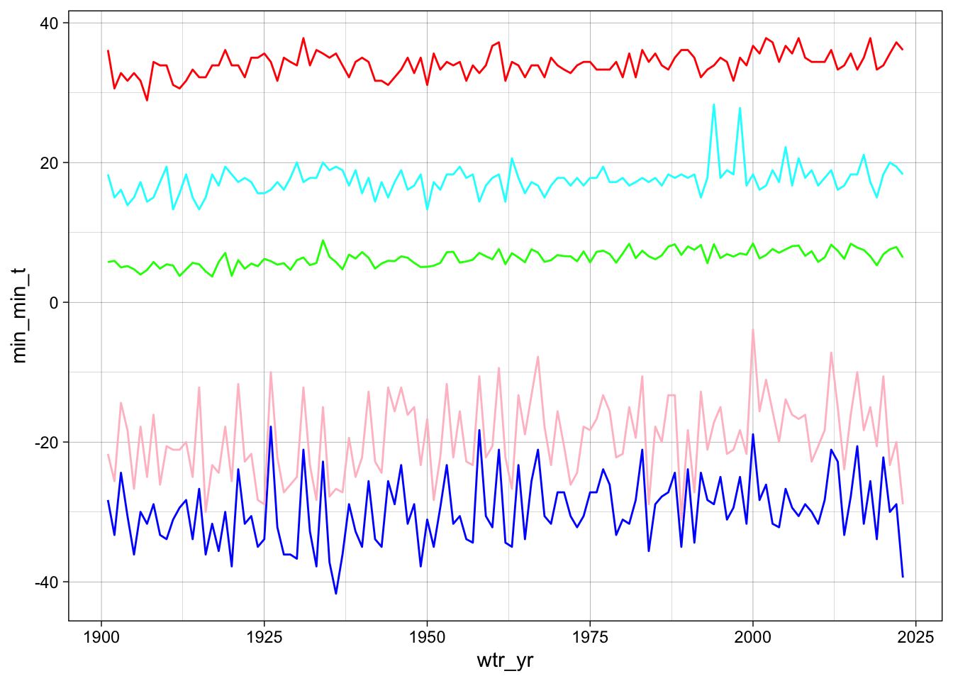
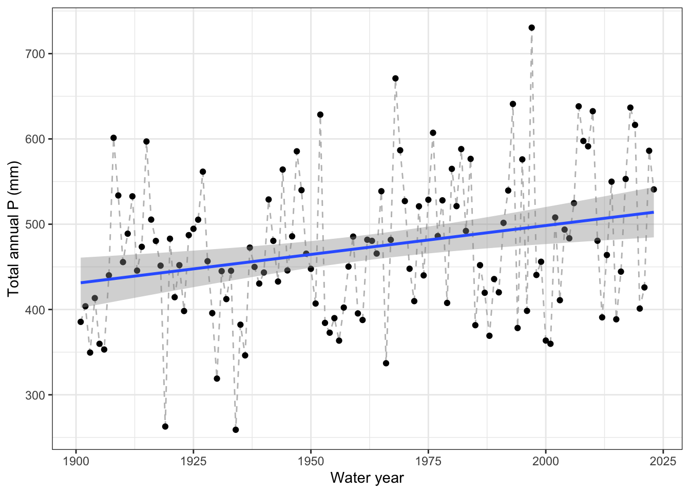
For your own insight, make plots of the variables in met_data_an over time to see if there appear to be trends in any of the data.

If you want practice making a function you can do so here. Remember functions look like:

my_fun <- function(x){ do_stuff() }

Can also be written as

my_fun <- function(…){ do_stuff() }

met_data_an %>% 
  ggplot(aes(x = wtr_yr)) +
  geom_line(aes(y = min_min_t), color = "blue") +
  geom_line(aes(y = max_min_t), color = "cyan") +
  geom_line(aes(y = min_max_t), color = "pink") +
  geom_line(aes(y = max_max_t), color = "red") +
  geom_line(aes(y = av_t), color = "green") 

met_data_an %>% 
  ggplot(aes(x = wtr_yr, y = tot_p)) +
  geom_line(linetype = "dashed", color = "grey") +
  geom_point() +
  geom_smooth(method = "lm") +
  labs(y = "Total annual P (mm)", x = "Water year") +
  theme_bw()

14.6 Trend analysis and creating Table 1

Next, you will fill in a table. The table will have columns for:

• See the word doc handout for an example of the table that you will fill in.

• total annual prcp

• the min of the minimum temperatures

• the max of the minimum temperatures

• the min of the maximum temperatures

• the max of the maximum temperatures

• the mean of the average temperatures

And values for:

• the p-value for the Mann-Kendall test. We will use p < 0.05 as an indicator of a significant trend.

• the slope of the trend as given by the Sen’s slope.

t_sens_tot_p <- sens.slope(met_data_an$tot_p) # this is how you would get the MK p-value and Sen's slope for one of the variables (av_t) in the data frame. Can you use apply or map to do this for all the variables in the data frame?  

t_sens_tot_p[3]

Both apply and map return a list. “A list in R can contain many different data types inside it. A list is a collection of data which is ordered and changeable.”

Here is a link with information about lists and how to access elements within the list https://data-flair.training/blogs/r-list-tutorial/

Chapters 19 & 21 in RDS are both very useful resources for functions and iteration (e.g., apply, map).

In the next class I will show a tutorial on apply, map and pulling information from lists. But you should work with a partner to test them out and see what they do.

met_test_data <- met_data_an %>% 
  filter(wtr_yr > 1989 & wtr_yr < 2021) %>% 
  select(-wtr_yr)

test <- apply(X = met_test_data,    # The data frame you want to apply to
      FUN = sens.slope,           # The function you want to run
      MARGIN = 2)                 # Margin (axis) to apply over 1 = rows, 2 = columns

test[[c(1,1)]]

test_map <- met_test_data %>% 
  map(sens.slope)

#Extract values from the list manually. 

test_map[[c(1,3)]]

#Extract values from the list using map. This part does the p-values. 
p_vals <- test_map[1:6] %>% 
  map(3) %>%
  flatten_dfc() %>% 
  pivot_longer(names_to = "parameter", 
               values_to = "p_value",
               cols = everything())

#Same as above but for Sens's slopes. 
sens <- test_map[1:6] %>% 
  map(1) %>%
  flatten_dfc() %>% 
  pivot_longer(values_to = "sens_slope",
               cols = everything()) %>% 
  select(-name)
  
  
#Last, we bind the two data frames together so we have the p-values and the Sen's slopes both in one df. 
sens_p <- cbind(p_vals, sens)

14.7 See summary section at top for questions to answer and deliverable.