Chapter 4 Snowmelt Models for runoff timing - Lecture & Lab (20 pts)
4.1 Module repo
4.2 Background:
Understanding snowmelt runoff is crucial for managing water resources and assessing flood risks, as it plays a significant role in the hydrologic cycle. Annual runoff and peak flow are influenced by snowmelt, rainfall, or a combination of both. In regions with a snowmelt-driven hydrologic cycle, such as the Rocky Mountains, snowpack acts as a natural reservoir, storing water during the winter months and releasing it gradually during the spring and early summer, thereby playing a vital role in maintaining water availability for various uses downstream. By examining how snowmelt interacts with other factors like precipitation, land cover, and temperature, we can better anticipate water supply fluctuations and design effective flood management strategies.
Learning objectives:
In this module, our primary focus will be modeling snowmelt as runoff, enabling us to predict when it will impact streamflow timing. We will consider some factors that may influence runoff timing. However, the term ‘snowmelt modeling’ is a field in itself and can represent a lifetime worth of work. There are many uses for snowmelt modeling (e.g., climate science and avalanche forecasting). If you are interested in exploring more on this subject, there is an excellent Snow Hydrology: Focus on Modeling series offered by CUAHSI’s Virtual University on YouTube.
Helpful terms:
The most common way to measure the water content of the snowpack is by the Snow Water Equivalent or SWE. The SWE is the water depth resulting from melting a unit column of the snowpack.
4.3 Model Approaches
Similar to the model development structure we discussed in the last module, snowmelt models are generally classified into three different types of abalation algorithms
Empirical and Data-Driven Models: These models use historical data and statistical techniques to predict runoff based on the relationship between snow characteristics (like snow area) and runoff. They use past patterns to make predictions about the future. The emergence of data-driven models has benefited from the growth of massive data and the rapid increase in computational power. These models simulate the changes in snowmelt runoff using machine learning algorithms to select appropriate parameters (e.g., daily rainfall, temperature, solar radiation, snow area, and snow water equivalent) from different data sources.
Conceptual Models: These models simplify the snowmelt process by establishing a simple, rule-based relationship between snowmelt and temperature. These models use a basic formula based on temperature to estimate how much snow will melt.
Physical Models: The physical snowmelt models calculate snowmelt based on the energy balance of snow cover. If all the heat fluxes toward the snowpack are considered positive and those away are considered negative, the sum of these fluxes is equal to the change in heat content of the snowpack for a given time period. Fluxes considered may be
- net solar radiation (solar incoming minus albedo),
- thermal radiation,
- sensible heat transfer of air (e.g., when air is a different temperature than snowpack),
- latent heat of vaporization from condensation or evaporation/sublimation, heat conducted from the ground,
- advected heat from precipitation
examples: layered snow thermal model (SNTHERM) and physical snowpack model (SNOWPACK),
Many effective models may incorporate elements from some or all of these modeling approaches.
4.4 Spatial complexity
We may also identify models based on the model architecture or spatial complexity. The architecture can be designed based on assumptions about the physical processes that may affect the snowmelt to runoff volume and timing.
Homogenous basin modeling: You may also hear these types of models referred to as ‘black box’ models. Black-box models do not provide a detailed description of the underlying hydrological processes. Instead, they are typically expressed as empirical models that rely on statistical relationships between input and output variables. While these models can predict specific outcomes effectively, they may not be ideal for understanding the physical mechanisms that drive hydrological processes. In terms of snow cover, this is a simplistic case model where we assume:
- the snow is consistent from top to bottom of the snow column and across the watershed
- melt appears at the top of the snowpack
- water immediately flows out the bottom
This type of modeling may work well if the snowpack is isothermal, if we are interested in runoff over large timesteps, or if we are modeling annual water budgets in lumped models.
Vertical layered modeling: Depending on the desired application of the model, snowmelt may be modeled in multiple layers in the snow column (air-snow surface to ground). Climate models, for example, may estimate phase changes or heat flux and consider the snowpack in 5 or more layers. Avalanche forecasters may need to consider grain evolution, density, water content, and more over hundreds of layers! Hydrologists may also choose variable layers, but many will choose single- or two-layer models for basin-wide studies, as simple models can be effective when estimating basin runoff. Here is a study by Dutra et al. (2012) that looked at the effect of the number of snow layers, liquid water representation, snow density, and snow albedo parameterizations within their tested models. Table 1 and figures 1-3 will be sufficient to understand the effects of changes to these parameters on modeled runoff and SWE. In this case, the three-layer model performed best when predicting the timing of the SWE and runoff, but density improved more by changing other parameters rather than layers (Figure 1).
Lateral spatial heterogeneity: The spatial extent of the snow cover determines the area contributing to runoff at any given time during the melt period. The more snow there is, the more water there will be when it melts. Therefore, snow cover tells us which areas will contribute water to rivers and streams as the snow melts. In areas with a lot of accumulated snow, the amount of snow covering the ground gradually decreases as the weather warms up. This melting process can take several months. How quickly the snow disappears depends on the landscape. For example, in mountainous ecosystems, factors like elevation, slope aspect, slope gradient, and forest structure affect how the snow can accumulate, evaporate or sublimate and how quickly the snow melts.
For mountain areas, similar patterns of depletion occur from year to year and can be related to the snow water equivalent (SWE) at a site, accumulated ablation, accumulated degree-days, or to runoff from the watershed using depletion curves from historical data. Here is an example of snow depletion curves developed using statistical modeling and remotely sensed data. The use of remotely sensed data can be incredibly helpful to providing estimates in remote areas with infrequent measurements. Observing depletion patterns may not be effective in ecosystems where patterns are more variable (e.g., prairies). However, stratified sampling with snow surveys, snow telemetry networks (SNOTEL) or continuous precipitation measurements can be used with techniques like cluster analyses or interpolation, to determine variables that influence SWE and estimate SWE depth or runoff over heterogeneous systems.
You can further explore all readings linked in the above section. These readings may assist in developing the workflow for your term project, though they are optional for completing this assignment. However, it is recommended that you review the figures to grasp the concepts and retain them for future reference if necessary.
4.5 Model choices: My snow is different from your snow
When determining the architecture of your snow model, your model choices will reflect the application of your model and the processes you are trying to represent. Recall that parsimony and simplicity often make for the most effective models. So, how do we know if we have a good model? Here are a few things we can check to validate our model choices:
Model Variability: A good model should produce consistent results when given the same inputs and conditions. Variability between model runs should be minimal if the watershed or environment is not changing.
Versatility: Check the model under a range of scenarios different from the conditions under which it was developed. The model should apply to similar systems or scenarios beyond the initial scope of development
Sensitivity Analysis: We reviewed this a bit in the Monte Carlo module. How do changes in model inputs impact outputs? A good model will show reasonable sensitivity changes in input parameters, with outputs responding as expected.
Validation with empirical data: Comparison with real-world data checks whether the model accurately represents the actual system
Applicability and simplicity: A good model should provide valuable insights or aid in decision-making processes relevant to the problem it addresses. It strikes a balance between complexity and simplicity, avoiding unnecessary intricacies that can lead to overfitting or computational inefficiency while sufficiently capturing the system’s complexities.
4.6 Codework
4.6.1 Download the repo for this lab HERE
In this module, we will simulate snowmelt in a montane watershed in central Colorado with a simple temperature model. The Fool Creek watershed is located in the Fraser Experimental Forest (FEF), 137 km west of Denver, Colorado. The FEF contains several headwater streams (Strahler order 1-3) within the Colorado Headwaters watershed which supplies much of the water to the populated Colorado Front Range. This Forest has been the site of many studies to evaluate the effects of land cover change on watershed hydrology. The Fool Creek is a small, forested headwater stream, with an approximate watershed area of 2.75 km^2. The watershed elevation ranges from approximately 2,930m (9,600ft) at the USFS monitoring station to 3,475m (11,400ft) at the highest point. There is a SNOTEL station located at 3,400m.
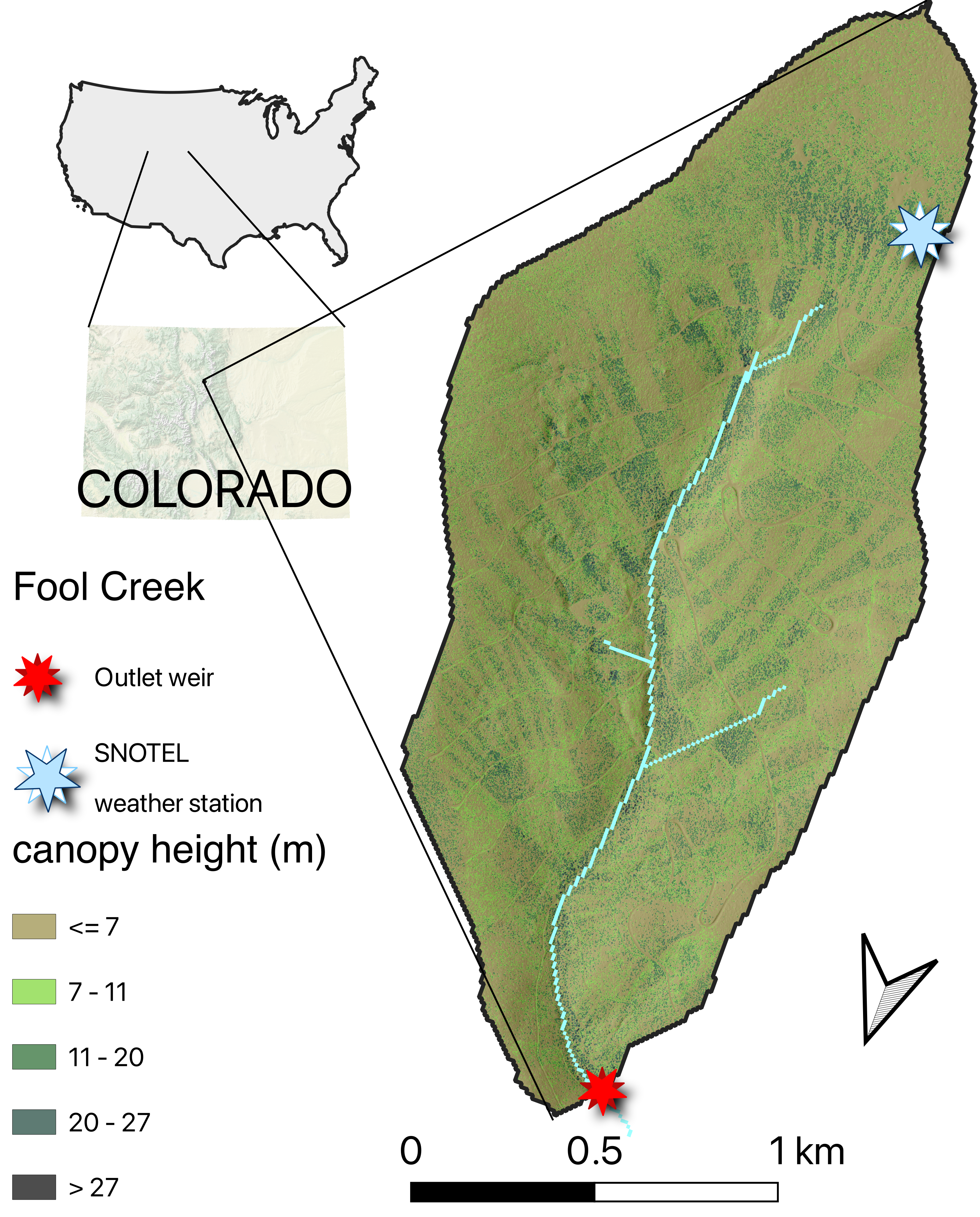
Question 1: Using this map, what differences can you see between these two sites or what variation do you see in the watershed that may affect snow accumulation and melt? (2 points)?
ANSWER:
Let’s look at some data for Fool Creek:
This script collects SNOTEL input data using snotelr. The SNOTEL automated collection site in Fool Creek supplies SWE data that can simplify our runoff modeling. Lets explore the sites available through snotelr and select the site of interest.
4.6.2 Import data:
We will generate a conceptual runoff model using the date, daily mean temperature, SWE depth in mm, and daily precipitation (mm). We will use select() to keep the desired columns only. Then we will use mutate() to add a water year, and group_by() to add a cumulative precipitation column for each water year.
# # Let's download data for the water years 2021 to 2022:
# df <- snotel_download(site_id = 1186, internal = TRUE) %>%
#     mutate(date = lubridate::ymd(date)) %>% # format the date
#     filter(between(date, lubridate::ymd("2020-10-01"), lubridate::ymd("2022-09-30"))) %>% # select desired dates
#     rename(swe.mm = snow_water_equivalent, # rename columns for easier use
#          precip.mm  = precipitation,
#          temp_mean.c = temperature_mean) %>%
#     # only select data we need
#     select(date, swe.mm, precip.mm, temp_mean.c) %>%
#     mutate(wtr_yr = if_else(month(date) < 10, year(date), year(date) + 1)) %>%
#     group_by(wtr_yr) %>% # add a water year column
#     mutate(pcumul.mm = cumsum(precip.mm)) %>% # generate a cumulative sum column for each water year
#     ungroup()
We will also download flow data collected by USFS at the Fool Creek outlet at 2,930m.
# fool_q <- read.csv("LFC_weir WY21-WY22.csv") %>%
#   mutate(date = mdy_hm(TIMESTAMP)) %>%
#   # convert cubic feet per second to metric (m/s^3)
#   # 1 cfs is equal to 0.028316847 cubic meter/second
#   mutate(m3_s = Q..cfs.*0.028316847)
Let’s look at the data for the SNOTEL station at 3400m in elevation.
# Plot imported SWE, precip and depth data data
# ggplot(data = df) +
#   geom_line(aes(x = date, y = swe.mm, color = 'swe.mm')) +
#   geom_line(aes(x = date, y = pcumul.mm, color = 'pcumul.mm')) +
#   geom_line(aes(x=date, y = precip.mm, color = 'precip.mm')) +
#   theme(axis.text.x = element_text(angle = 45, hjust = 1), # Rotate x-axis labels by 45 degrees
#         axis.line = element_line(color = "black"),  # Add black axis lines
#         panel.background = element_rect(fill = "white"),  # Set panel background to white
#         panel.grid.major = element_blank(),  # Remove major grid lines
#         panel.grid.minor = element_blank()) + # Remove minor grid lines
#   ylab("mm") +
#   xlab('Date')
4.6.3 Calculate liquid input
to the ground by analyzing the daily changes in Snow Water Equivalent (SWE) and precipitation. This script incorporates temperature conditions to determine when to add changes to liquid input.
# sntl <- df
#
# sntl <- sntl %>%
#   # calculate differences for SWE and cumulative P and put 0 as the first value
#   mutate(SWEdiff.mm = c(0, diff(sntl$swe.mm, lag = 1)), #find daily change in SWE
#         Pdiff.mm = c(0, diff(pcumul.mm, lag = 1))) %>%
#   # remove the negative values at the start of each year
#   mutate(Pdiff.mm = if_else(Pdiff.mm < 0, 0, Pdiff.mm)) %>%
#   # conditional statements for calculate liquid input to the ground
#   mutate(input.mm = if_else(Pdiff.mm > 0 & SWEdiff.mm, 0, 0),
#          input.mm = if_else(Pdiff.mm == 0 & SWEdiff.mm < 0, -SWEdiff.mm, input.mm),
#          input.mm = if_else(Pdiff.mm > 0 & SWEdiff.mm < 0, Pdiff.mm - SWEdiff.mm, input.mm),
#          input.mm = if_else(Pdiff.mm > 0 & SWEdiff.mm == 0, Pdiff.mm, input.mm)) %>%
#   # this replaces missing air temp values with 0
#   mutate(temp_mean.c = replace_na(temp_mean.c, 0)) %>%
#   # this is a check that prevents liquid inputs when the air temp is below 0
#   mutate(input.mm = if_else(temp_mean.c < 0 & input.mm > 0, 0, input.mm)) %>%
#   mutate(date = lubridate::ymd(date))
Question 2: In plain language, explain each step of the 5 if-else statements above (~5 brief sentences) (3pts).
ANSWER:
# # Create a cumulative input column for visualization and calculations
# sntl <- sntl %>%
#   group_by(wtr_yr) %>%
#   mutate(cum_input.mm = cumsum(input.mm)) %>% # generate a cumulative sum column for each water year
#   ungroup()
Let’s visualize the timing disparities between precipitation and melt input in relation to discharge.
# # Convert date column to POSIXct format
# fool_q$date <- as.POSIXct(fool_q$date)
# sntl$date <- as.POSIXct(sntl$date)
#
# # Plot imported SWE, precip, and depth data
# ggplot() +
#   # Scale discharge for the right y-axis
#   geom_line(data = fool_q, aes(x = date, y = m3_s*10000, color = 'm^3/second')) +
#   geom_point(data = sntl, aes(x = date, y = cum_input.mm, color = 'cumulative input (mm)')) +
#   geom_point(data = sntl, aes(x = date, y = pcumul.mm, color = 'cumulative precipitation (mm)')) +
#   theme(axis.text.x = element_text(angle = 45, hjust = 1), # Rotate x-axis labels by 45 degrees
#         axis.line = element_line(color = "black"),  # Add black axis lines
#         panel.background = element_rect(fill = "white"),  # Set panel background to white
#         panel.grid.major = element_blank(),  # Remove major grid lines
#         panel.grid.minor = element_blank(), # Remove minor grid lines
#         ) +
#   ylab("mm") +
#   xlab('Date') +
# scale_y_continuous(sec.axis = sec_axis(trans = ~ . / 10000, name = expression(Q[paste(m^3,'/second')])))Question 3. What processes could account for the differences between cumulative input, calculated from SWE data, and cumulative precipitation, both measured at the same SNOTEL station? (1 or 2 processes) What could explain the discrepancy if the cumulative input, is found to be less than the cumulative precipitation measured at the same SNOTEL station? (at least 2 possible processes) (4 points) (2-3 sentences)
ANSWER:
4.7 Modeling SWE
Let’s assume that we have a precipitation gage at 3400m in Fool Creek, but without SWE data, how could we model SWE using temperature?
# # Filter to a single water year for the snowmelt model
# wateryr = '2021'
#
# # set the year
# sntl_SINGLE_YEAR <- sntl %>%
#   filter(wtr_yr == wateryr)
#
# print(sum(sntl_SINGLE_YEAR$input.mm))
The model below is a variation of the degree-day method. Here we are running a similar script to the input calculations above, using temperature as the primary determinant. When the temperature falls below a certain threshold and precipitation occurs, an equivalent amount is added to our SWE accumulation. We’ll conduct a simulation with 100 Monte Carlo runs and analyze the optimal outcome. The parameters we are testing are pack threshold, a degree-day factor, and the threshold temperature for determining rain from snow.
# ########################################
# # nx sets the number of Monte Carlo runs
# nx <- 100 # number of runs
#
# # set up the parameter matrix
# param <- tibble(
#   Run = vector(mode = "double", nx),
#   ddf = vector(mode = "double", nx),
#   Tb = vector(mode = "double", nx),
#   pack_threshold = vector(mode = "double", nx),
#   nse = vector(mode = "double", nx),
#   kge = vector(mode = "double", nx),
#   SWEsim = vector(mode = "list", nx)
# )
#
# tic("MC Simulation")
# pb <- progress_bar$new(
#   format = " downloading [:bar] :percent eta: :eta",
#   total = nx, clear = FALSE, width = 60
# ) # initialize progress bar
#
# #### MONTE CARLO SETUP (use ii as index)
# for (n in 1:nx) {
#   pb$tick() # needed for progress bar
#
#   # write run number into the parameter matrix
#   param$Run[n] <- n
#
# #####################
# # initiate parameters
#   param$ddf[n] <- runif(1, 0, 5) # Threshold temperature for distinguishing rain from snow.
#   param$Tb[n] <- runif(1, -5, 5) # Degree-day factor for snowmelt calculations, utilized in calculating the potential melt (Melt) based on the difference between the mean temperature (temp_mean.c) and Tb.
#   param$pack_threshold[n] <- runif(1, 0, 100) #threshold value used in determining whether precipitation falls as snow or accumulates on existing snowpack
#
# ########################################
# # generate columns with snow, rain, melt
#   SWE.Model <- sntl_SINGLE_YEAR %>%
#     # liquid precipitation
#     mutate(Rain = if_else(Pdiff.mm > 0 & temp_mean.c >= param$Tb[n], Pdiff.mm, 0)) %>%
#    # snow accumulation
#     mutate(Snow = if_else(Pdiff.mm > 0 & temp_mean.c < param$Tb[n], Pdiff.mm, 0)) %>%
#   # potential melt
#     mutate(Melt = if_else(temp_mean.c > param$Tb[n], param$ddf[n]*(temp_mean.c - param$Tb[n]), 0)) %>%
#   # cumulative SWE without melt
#     mutate(SWE.cumul = cumsum(Snow)) %>%
#   # no melt if swe <= 0 (here only for first few steps)
#      mutate(Melt = if_else(SWE.cumul == 0, 0, Melt))
#
#
# ########################################
# # for loop to loop through each timestep
#   SWEsim <- vector()
#   SWEsim[1] <- 0 # set first value to 0
#   for (ii in 2:dim(SWE.Model)[1]) {
#
#   # snow accumulation if snowfall happens
#     SWEsim[ii] <- if_else(SWE.Model$Snow[ii] > 0, SWE.Model$Snow[ii]+SWEsim[ii-1],
#
# #This condition checks if the existing snow water equivalent (SWE) surpasses the pack threshold. If so, then the precipitation is considered to contribute to the snowpack rather than falling as rain
#   # snow accumulation if liquid precip but snow on the ground
#     if_else(SWE.Model$Rain[ii] > 0 & SWEsim[ii-1] > param$pack_threshold[n], SWE.Model$Rain[ii]+SWEsim[ii-1],
#
#   # melt if SWEsim on the ground larger than the melt pulse
#     if_else(SWE.Model$Melt[ii] > 0 & SWEsim[ii-1] > SWE.Model$Melt[ii], SWEsim[ii-1] - SWE.Model$Melt[ii],
#
#   # melt if SWEsim is present but smaller than melt pulse
#   if_else(SWE.Model$Melt[ii] > 0 & SWEsim[ii-1] < SWE.Model$Melt[ii], 0, SWEsim[ii-1]))))
# }
#
# # store simulated SWEsim in df
# param$SWEsim[n] <- list(SWEsim)
#
#
# ####################
# # We will store efficiencies comparing observed SWE with simulated SWE.
# # NSE
#     param$nse[n] <- 1 - ((sum((SWE.Model$swe.mm - SWEsim)^2)) / sum(((SWE.Model$swe.mm - mean(SWE.Model$swe.mm))^2)))
#
#     # KGE
#     kge_r <- cor(SWE.Model$swe.mm, SWEsim)
#     kge_beta <- mean(SWEsim) / mean(SWE.Model$swe.mm)
#     kge_gamma <- (sd(SWEsim) / mean(SWEsim)) / (sd(SWE.Model$swe.mm) / mean(SWE.Model$swe.mm))
#     param$kge[n] <- 1 - sqrt((kge_r - 1)^2 + (kge_beta - 1)^2 + (kge_gamma - 1)^2)
#
#
# }
# toc()
#
# #########################################
# # sort parameter matrix from highest to lowest NSE and save it
# param <- arrange(param, desc(nse))
# save(param, file = paste(wateryr, "SWE.Model.Runs.RData", sep = "."))
#
# # best run
# # take the best run, get the list of simulated values and unlist it in order to store it in a dataframe
# SWE.Model$SWEsim.mm <- unlist(param$SWEsim[1])
# # Plot best run
# swe_plot <- ggplot(data = SWE.Model) +
# geom_line(aes(x = date, y = SWEsim.mm, color = "Simulated SWE")) +
# geom_line(aes(x = date, y = swe.mm, color = "Actual SWE")) +
# annotate("text", x = mean(SWE.Model$date, na.rm = TRUE), y = min(SWE.Model$swe.mm, na.rm = TRUE),
# label = paste("NSE =", round(param$nse[1], 2)), hjust = 1, vjust = 1)
#
# ggplotly(swe_plot)This simple model seems to simulate SWE well if assessed with the NSE. Let’s model SWE at the Fool Creek outlet, where we do not have daily SWE data. First we’ll bring in precipitation data, measured at a USFS maintained meteorological station located near the Fool outlet:
# fc_precip <- read.csv("LFCmet_WY21_WY22.csv") %>%
#   mutate(date = lubridate::mdy_hm(TS)) %>%
#   select(date, water_year, PPT_10min..mm.) %>%
#   filter(water_year %in% c(2021, 2022))
We also need temperature data. This is also collected at the USFS Lower Fool meteorological station.
# fc_temp <- read.csv("lfc_airtemp.csv") %>%
#   mutate(date = lubridate::mdy_hm(TMSTAMP)) %>%
#   mutate(wtr_yr = if_else(month(date) < 10, year(date), year(date) + 1)) %>%
#   select(date, Air_TempC_Avg, wtr_yr) %>%
#   filter(wtr_yr %in% c(2021, 2022))
#
# lfc_data <- merge(fc_temp, fc_precip, by = "date", validate = "one_to_one") %>%
#   select(date, Air_TempC_Avg, wtr_yr, PPT_10min..mm.) %>%
#   rename(precip.mm  = PPT_10min..mm.,
#          temp_mean.c = Air_TempC_Avg)
#   # rename columns so we can reuse the SWE model without changing variable names within the simulation code
#
# # Lets add cumulative precip totals by water year
# lfc_data <- lfc_data %>%
#   group_by(wtr_yr) %>%
#   mutate(pcumul.mm = cumsum(precip.mm)) %>% # generate a cumulative sum column for each water year
#   ungroup()
#
# # Aggregate all data to daily means for the sake of simulation time
# lfc_data <- lfc_data %>%
#   group_by(date = as.Date(date)) %>%
#   summarise(across(.cols = everything(), .fns = mean, na.rm = TRUE))
Even though this meteorological station is very close to the SNOTEL station, lets compare the values between the upper watershed and the lower
# # Convert date column in sntl to Date format that matches lfc_data
# sntl$date <- as.Date(sntl$date)
#
# ggplot() +
#   # Scale discharge for the right y-axis
#   geom_point(data = lfc_data, aes(x = date, y = pcumul.mm, color = 'lower fool creek precip (mm)')) +
#   geom_point(data = sntl, aes(x = date, y = pcumul.mm, color = 'upper fool creek precip (mm)')) +
#   theme(axis.text.x = element_text(angle = 45, hjust = 1), # Rotate x-axis
#         panel.grid.minor = element_blank(), # Remove minor grid lines
#         ) +
#   ylab("mm") +
#   xlab('Date')
Now let’s estimate SWE for the Lower Fool Creek. Again, we’ll just simulate a single year.
# # Filter to a single water year for the snowmelt model
# wateryr = '2021'
#
# # aggregate data to daily means for the sake of simulation time
# lfc_data <- lfc_data %>%
#   mutate(Pdiff.mm = pcumul.mm - lag(pcumul.mm, default = first(pcumul.mm)))
#
# # set the year
# lfc_SINGLE_YEAR <- lfc_data %>%
#   filter(wtr_yr == wateryr)
Run another set of simulations and compare the values of the best performing parameters across sites.
# ########################################
# # nx sets the number of Monte Carlo runs
# nx <- 100 # number of runs
#
# # set up the parameter matrix
# param <- tibble(
#   Run = vector(mode = "double", nx),
#   ddf = vector(mode = "double", nx),
#   Tb = vector(mode = "double", nx),
#   pack_threshold = vector(mode = "double", nx),
#   nse = vector(mode = "double", nx),
#   kge = vector(mode = "double", nx),
#   SWEsim = vector(mode = "list", nx)
# )
#
# tic("MC Simulation")
# pb <- progress_bar$new(
#   format = " downloading [:bar] :percent eta: :eta",
#   total = nx, clear = FALSE, width = 60
# ) # initialize progress bar
#
# #### MONTE CARLO SETUP (use ii as index)
# for (n in 1:nx) {
#   pb$tick() # needed for progress bar
#
#   # write run number into the parameter matrix
#   param$Run[n] <- n
#
# #####################
# # initiate parameters
#   param$ddf[n] <- runif(1, 0, 5) # Threshold temperature for distinguishing rain from snow.
#   param$Tb[n] <- runif(1, -5, 5) # Degree-day factor for snowmelt calculations, utilized in calculating the potential melt (Melt) based on the difference between the mean temperature (temp_mean.c) and Tb.
#   param$pack_threshold[n] <- runif(1, 0, 100) #threshold value used in determining whether precipitation falls as snow or accumulates on existing snowpack
#
# ########################################
# # generate columns with snow, rain, melt
#   SWE.Modellfc <- lfc_SINGLE_YEAR %>%
#     # liquid precipitation
#     mutate(Rain = if_else(Pdiff.mm > 0 & temp_mean.c >= param$Tb[n], Pdiff.mm, 0)) %>%
#    # snow accumulation
#     mutate(Snow = if_else(Pdiff.mm > 0 & temp_mean.c < param$Tb[n], Pdiff.mm, 0)) %>%
#   # potential melt
#     mutate(Melt = if_else(temp_mean.c > param$Tb[n], param$ddf[n]*(temp_mean.c - param$Tb[n]), 0)) %>%
#   # cumulative SWE without melt
#     mutate(SWE.cumul = cumsum(Snow)) %>%
#   # no melt if swe <= 0 (here only for first few steps)
#      mutate(Melt = if_else(SWE.cumul == 0, 0, Melt))
#
#
# ########################################
# # for loop to loop through each timestep
#   SWEsim <- vector()
#   SWEsim[1] <- 0 # set first value to 0
#   for (ii in 2:dim(SWE.Modellfc)[1]) {
#
#   # snow accumulation if snowfall happens
#     SWEsim[ii] <- if_else(SWE.Modellfc$Snow[ii] > 0, SWE.Modellfc$Snow[ii]+SWEsim[ii-1],
#
#   # snow accumulation if liquid precip but snow on the ground
#     if_else(SWE.Modellfc$Rain[ii] > 0 & SWEsim[ii-1] > param$pack_threshold[n], SWE.Model$Rain[ii]+SWEsim[ii-1],
#
#   # melt if SWEsim on the ground larger than the melt pulse
#     if_else(SWE.Modellfc$Melt[ii] > 0 & SWEsim[ii-1] > SWE.Modellfc$Melt[ii], SWEsim[ii-1] - SWE.Modellfc$Melt[ii],
#
#   # melt if SWEsim is present but smaller than melt pulse
#   if_else(SWE.Modellfc$Melt[ii] > 0 & SWEsim[ii-1] < SWE.Modellfc$Melt[ii], 0, SWEsim[ii-1]))))
# }
#
# # store simulated SWEsim in df
# param$SWEsim[n] <- list(SWEsim)
#
#
# ####################
# # We will store efficiencies comparing observed SWE with simulated SWE.
# # NSE
#     param$nse[n] <- 1 - ((sum((SWE.Model$swe.mm - SWEsim)^2)) / sum(((SWE.Model$swe.mm - mean(SWE.Model$swe.mm))^2)))
#
#     # KGE
#     kge_r <- cor(SWE.Model$swe.mm, SWEsim)
#     kge_beta <- mean(SWEsim) / mean(SWE.Model$swe.mm)
#     kge_gamma <- (sd(SWEsim) / mean(SWEsim)) / (sd(SWE.Model$swe.mm) / mean(SWE.Model$swe.mm))
#     param$kge[n] <- 1 - sqrt((kge_r - 1)^2 + (kge_beta - 1)^2 + (kge_gamma - 1)^2)
#
#
# }
# toc()
#
# #########################################
# # sort parameter matrix from highest to lowest NSE and save it
# param_lfc <- arrange(param, desc(nse))
# # Can save simulated data if desired
# #save(param_lfc, file = paste(wateryr, "SWE_lfc.Model.Runs.RData", sep = "."))
#
#
# # take the best run, get the list of simulated values and unlist it in order to store it in a dataframe
# SWE.Modellfc$SWEsim.mm <- unlist(param_lfc$SWEsim[1])
Since we don’t have SWE measurement for Lower Fool Creek, let’s see how the simulated values compare to acutal Upper Fool SNOTEL SWE measurements.
# SWE.Model$date <- as.Date(SWE.Model$date)
# # Plot best run
# swe_plot <- ggplot() +
#   geom_line(data = SWE.Modellfc, aes(x = date, y = SWEsim.mm, color = "Simulated SWE")) +
#   geom_line(data = SWE.Model, aes(x = date, y = swe.mm, color = "Actual SWE")) +
#   annotate("text", x = mean(SWE.Model$date, na.rm = TRUE), y = min(SWE.Model$swe.mm, na.rm = TRUE),
#            label = paste("NSE =", round(param$nse[1], 2)), hjust = 1, vjust = 1)
#
# ggplotly(swe_plot)
# compare the best performing parameters for the Upper Fool Creek and Lower Fool Creek
# print(param[1, ])
# print(param_lfc[1, ])
#
# # You can change the indexing and wording in this statement if you want to explore all parameters.
# print(paste('The estimated threshold temperature distinguishing rain from snow in Lower Fool is ', round(param_lfc[1, 2], 2), 'degrees and in Upper Fool Creek is', round(param[1, 2],2), 'degrees'))Question 3: Based on the differences in precipitation and temperature totals between the two sites, are SWE simulation results as you expected? (1 sentence)(2pnts)
ANSWER:
Question 4: How does the estimated threshold temperature distinguishing rain from snow change with elevation? Is the relationship between your parameter estimations as expected? How does this influence your confidence in the model? (2pnts)
ANSWER
Question 4: Compare the precipitation and snow accumulation patterns between two sites. Discuss at least 3 potential natural and/or anthropogenic mechanisms driving the observed variations in precipitation and snow accumulation. Consider the factors you observed in question 1 (3 points)(2-3 sentences).
ANSWER:
Question 5: Let’s say you want to model runoff for the Fool Creek catchment identified above. To do that, you want to estimate the timing and volume of snowmelt for this watershed. Refer to at least 2 model types reviewed in the 06_model_classifications lecture or terms in the lecture above and qualitatively describe a model that you could use to capture the spatial heterogeneity of snow accumulation in this watershed (4 points) (2-4 sentences).
ANSWER: